Preparation for Unstacking

Data Preparation

Obtain Offline Data

The RVS developer community provides an unstacking offline project data package to help users quickly get started, validate functionality, and save time. Click unstacking_runtime.zip to download. After extraction, the contents include:

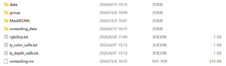
File Description

File	Description
data	This folder contains the Elite robot model used in this case. If you need other models, please visit the RVS software release model website to download.
group	This folder contains commonly used Group sets, including loading, hand-eye calibration conversion, etc. Import as needed.
MaskRCNN	The contents of this folder are used for AI inference. Among them, ty_ai_savedata.rvs is used for AI image recording, and ty_ai_train.rvs is used for AI training.
unstacking_data	This folder contains the offline data for the unstacking program. Please ensure the correct path is used when loading.
rgb2tcp.txt	This file contains the EyeInHand hand-eye calibration results for the Elite robot in this case.
ty_color/depth_calib.txt	This file contains the color camera calibration parameters and depth camera calibration parameters for the camera in this case.
unstacking.rvs	This project is used for the unstacking program and can be used as a reference. When loading offline data, please ensure the paths for TyCameraSimResource and LoadLocalTCP Group are correct.

All files used in this case are saved in the unstacking_runtime folder. Please place it in the RVS installation directory to run.

Note

Ensure the node file paths are correctly loaded during runtime. If you do not want to modify the file paths, you can place the files in the same directory as the running program.

This document uses RVS software version 1.8.321. If you encounter any issues or version incompatibility, please provide feedback promptly by sending an email to rvs-support@percipio.xyz!

Software Preparation

Download RVS_AI Software

For complex scenarios, you can download the RVS_AI software to re-annotate and train the AI model, and perform inference based on it.

Note

Please refer to the RVS Installation Tutorial to verify if your computer configuration meets the requirements for AI training.

The RVS_AI software download links are as follows:

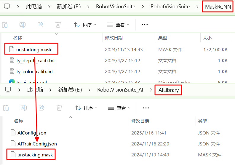
After extracting the downloaded file, RVS_AI_Center.exe in the folder is the RVS-AI executable file. The AILibrary folder stores the trained AI models for subsequent inference.
In this case, you need to move the unstacking.mask compressed file from the MaskRCNN folder in the unstacking offline project data package to the AILibrary folder.

Real Scene Operation

For real scene operations, prepare the real scene robot hand-eye calibration file and ensure the correct path is used during operation.

Unstacking Process

Overview of the Unstacking Process

The actual goal of automatic unstacking is to find the geometric center of the box and pick it up in a certain order. The specific unstacking process can be divided into the following steps:

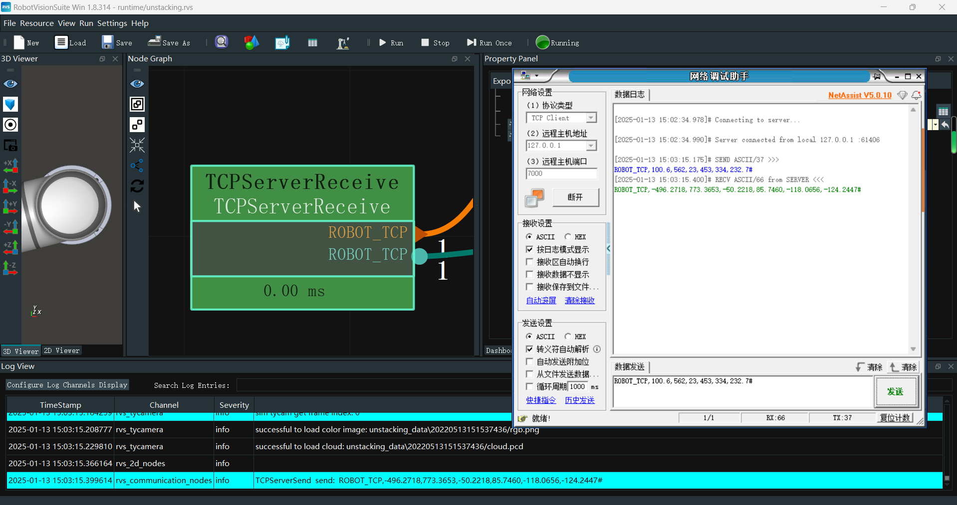
Communication Reception: Trigger the project based on the communication command sent by the robot.

The communication string format used in this case is “ROBOT_TCP,X,Y,Z,RX,RY,RZ#”. Here, X,Y,Z,RX,RY,RZ represent the robot TCP pose when capturing the image.
Load Local Data: This case uses offline data to complete the unstacking project.
Coordinate System Conversion: Convert the point cloud from the camera coordinate system to the robot coordinate system.
AI Inference and Point Cloud Segmentation: When boxes are tightly packed, use AI inference to segment the box point clouds.
Filtering and Positioning: Identify the target point cloud, filter and sort it, and then perform positioning.
Communication Sending: Send the target positioning pose to the robot.

The sent string format is “ROBOT_TCP,X,Y,Z,RX,RY,RZ#”. Here, X,Y,Z,RX,RY,RZ represent the target positioning pose.
Robot Picking: This case uses robot simulation for sequential unstacking and picking.

Unstacking Project Demonstration

Operation Process

Start the RVS_AI inference service.
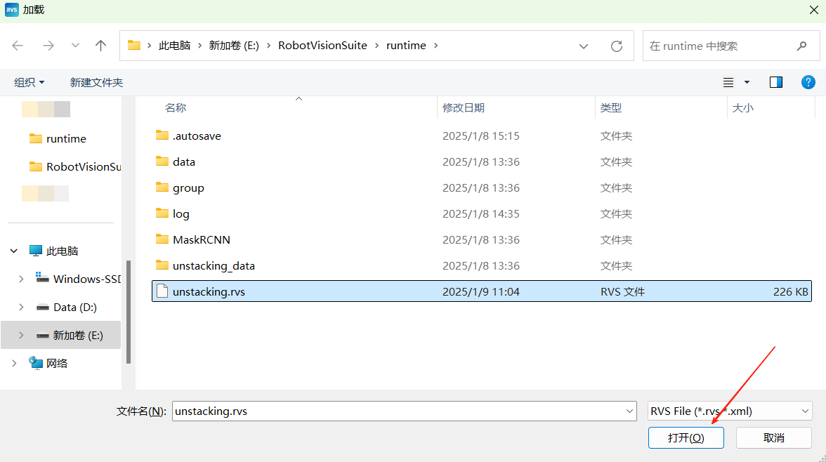
Open RVS and load the project.
- Click the load button, select unstacking.rvs, and open it.
Run the project.
- Click the RVS run button.
Trigger the project.
- Offline triggering.
  - Click the Offline Trigger button on the interaction panel to trigger.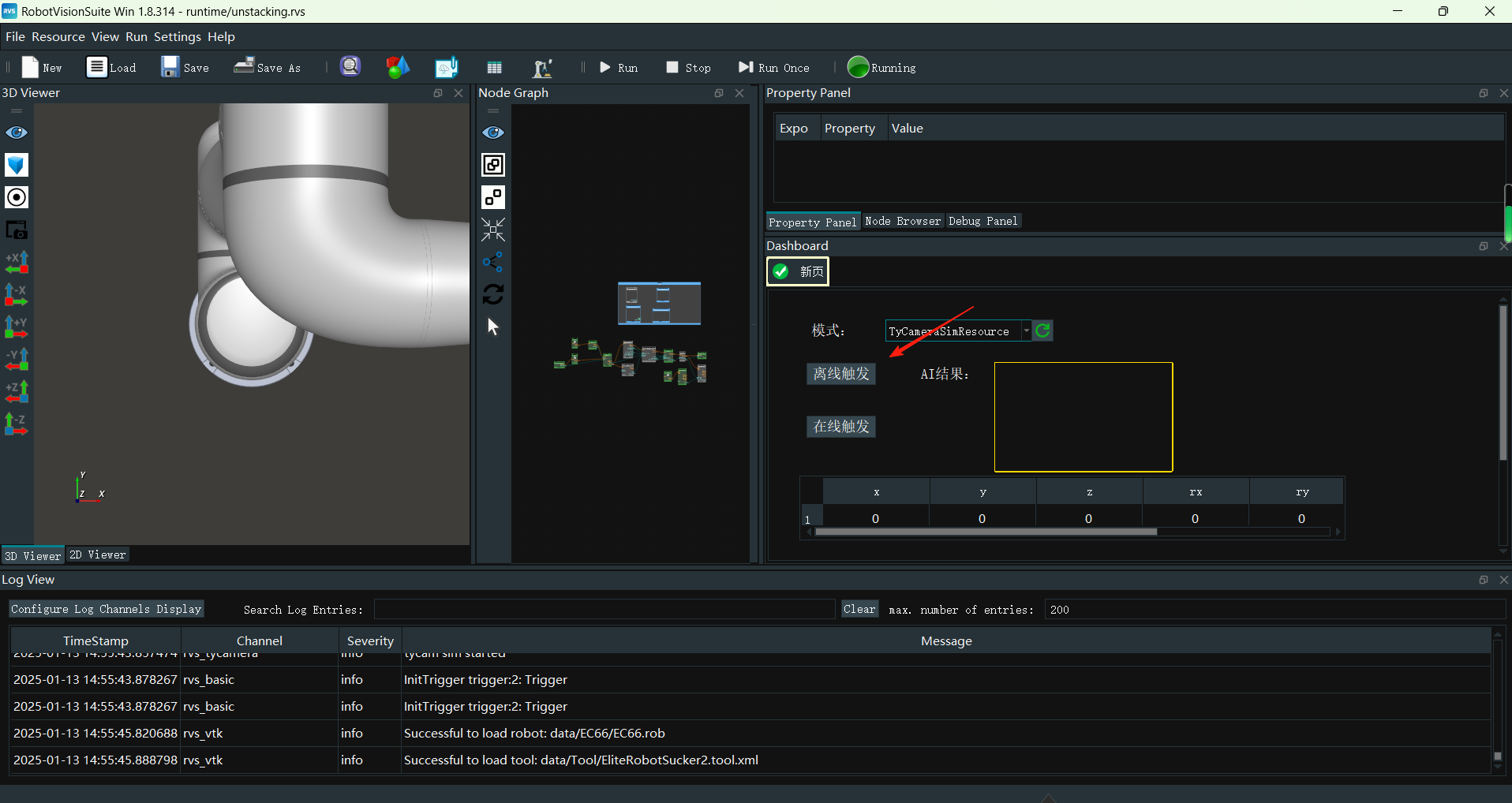
- Online triggering.
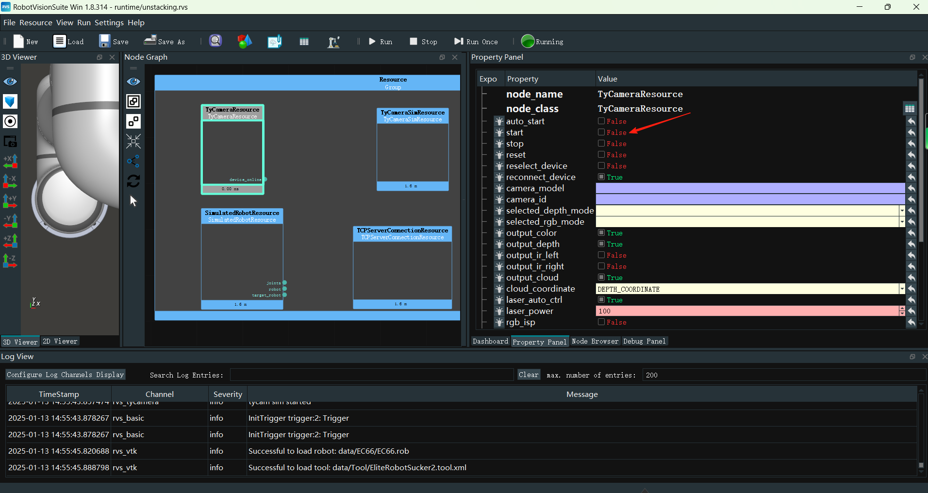
  - Connect the Tyto camera in the Resource Group.
    
    Note
    
    Auto Start: Automatically connect the Tyto camera when running the project.
    Start: Manually connect the camera after running the project.
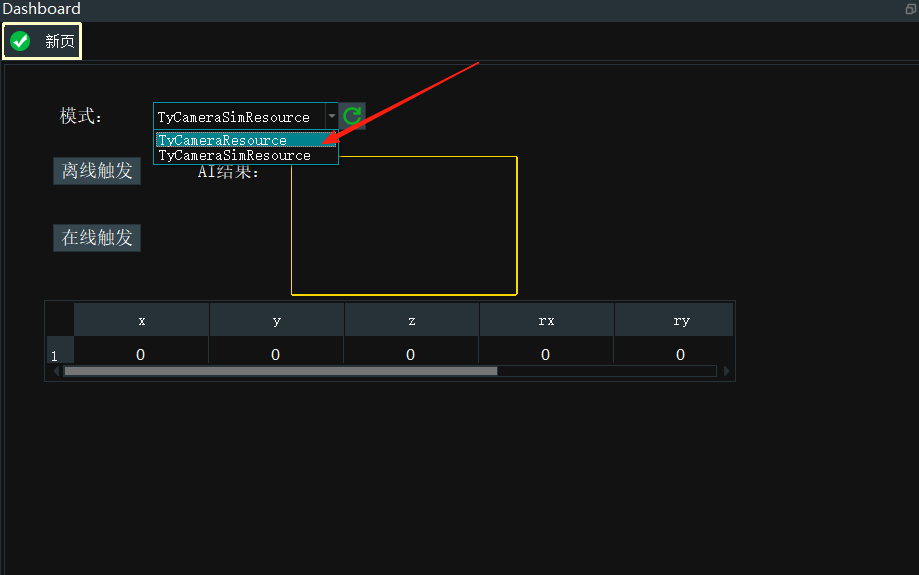
- Adjust the mode in the interaction panel, refresh the combo box, and select the Tyto camera resource.
- The robot sends “ROBOT_TCP,X,Y,Z,RX,RY,RZ#”. Here, X,Y,Z,RX,RY,RZ represent the robot TCP pose when capturing the image.
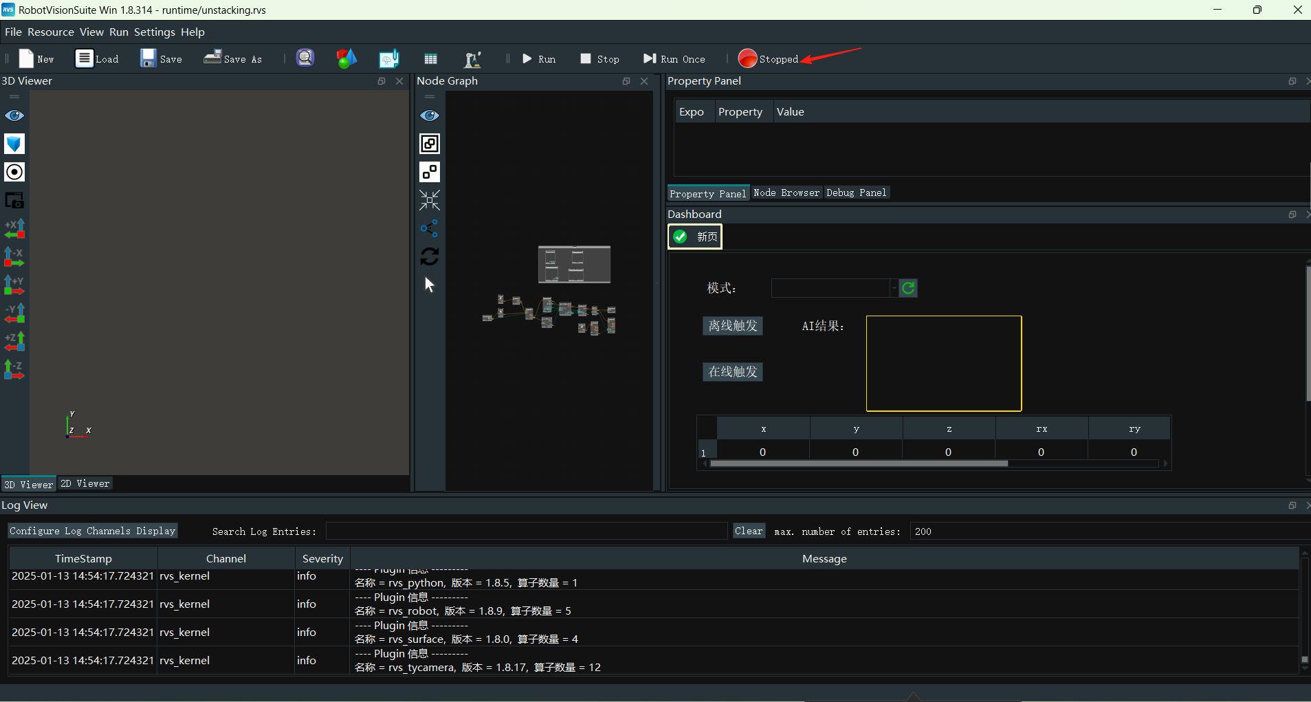
Run results.
- In offline mode, each time you click Offline Trigger, the robot performs sequential unstacking. In the 3D view, you can see the simulated robot’s picking pose. Check the AI results and specific pose information in the interaction panel.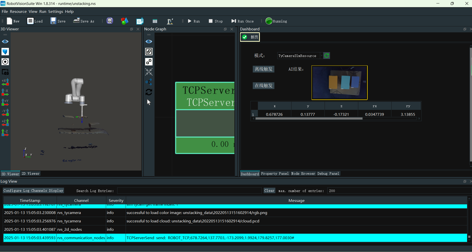

Unstacking Project Setup

Communication Reception

This case project is triggered by the communication command sent by the robot. This case uses the EyeInHand mode, requiring the current capture pose to be sent for calculation.

Operation Process

Create a new project and save it as unstacking.rvs.
Add the TCPServerConnectionResource node to the Resource Group to establish the TCP communication server.
- Set the TCPServerConnectionResource node parameters:
  - Auto Start → Yes
  - Port → 7000
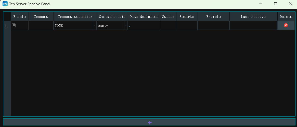
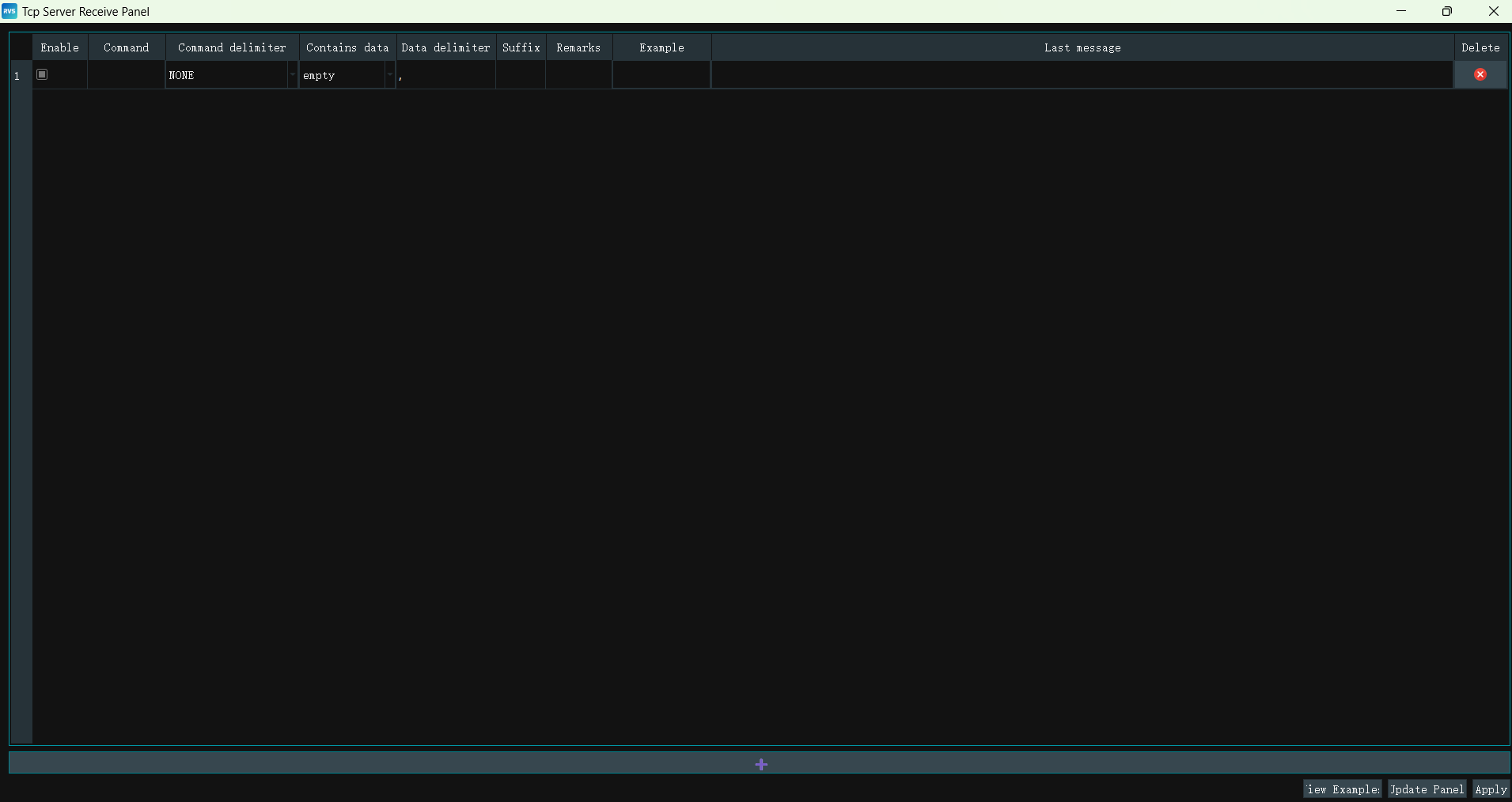
Add the TCPServerReceive node to the node diagram to trigger the project run via communication commands.
- Right-click the TCPServerReceive node and open the node panel:
  - Click
  - Command → ROBOT_TCP
  - Command Separator → ,
  - Include Data → pose
  - Data Separator → ,
  - Suffix → #
The TCPServerReceive node panel configuration is as follows:

Offline/Online Data

In this case, the offline data is in the unstacking_data folder, containing point clouds, joints, 2D images, and TCP. Online data requires connecting the Tyto camera and robot communication to obtain real-time data.

Note

If you need to perform the unstacking process based on the actual scene, connect the camera and camera resource to complete online unstacking.

Operation Process

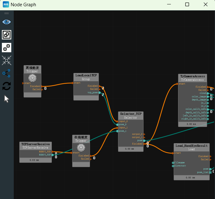
Add two Trigger nodes to the node diagram to trigger offline/online project runs.
- Set Trigger node parameters:
  - node_name → Offline Trigger
- Set Trigger_0 node parameters:
  - node_name → Online Trigger
Import the LoadLocalTCP.group from the group folder to traverse offline robot TCP data.
- Set LoadLocalTCP.group parameters:
  - Parent Directory → unstacking_data
Note

Note the runtime path of this project.
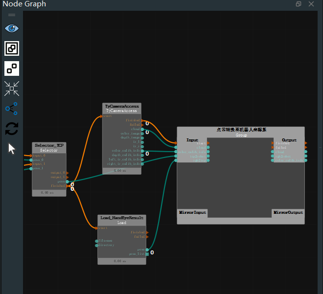
Add the Selector node to the node diagram to select offline or online robot TCP data for subsequent calculations.
- Set Selector node parameters:
  - node_name → Selector_TCP
  - Type → Coordinate
Add TyCameraResource and TyCameraSimResource nodes to the Resource Group. TyCameraResource is used to connect the Tyto camera, and TyCameraSimResource is used to traverse offline point clouds, color images, depth images, etc.
- Set TyCameraSimResource node parameters:
  - Auto Start → Yes
  - Load Mode → Directory
  - Directory → unstacking_data
  - Color Image File → rgb.png
  - Depth Image File → depth.png
  - Point Cloud File → cloud.pcd
  - Depth Calibration File → ty_depth_calib.txt
  - Color Calibration File → ty_color_calib.txt
Note

Note the runtime path of this project.
- Set TyCameraResource node parameters:
  - Configure according to the actual Tyto camera.
Add the TyCameraAccess node to the node diagram to output point clouds, color images, depth images, etc.
- Set TyCameraAccess node parameters:
  - Camera Resource → TyCameraSimResource
Add the Load node to the node diagram to load the hand-eye calibration results.
- Set Load node parameters:
  - node_name → Load_HandEyeResult
  - Type → Coordinate
  - File → rgb2tcp.txt
Note

Note the runtime path of this project.
Connection node.
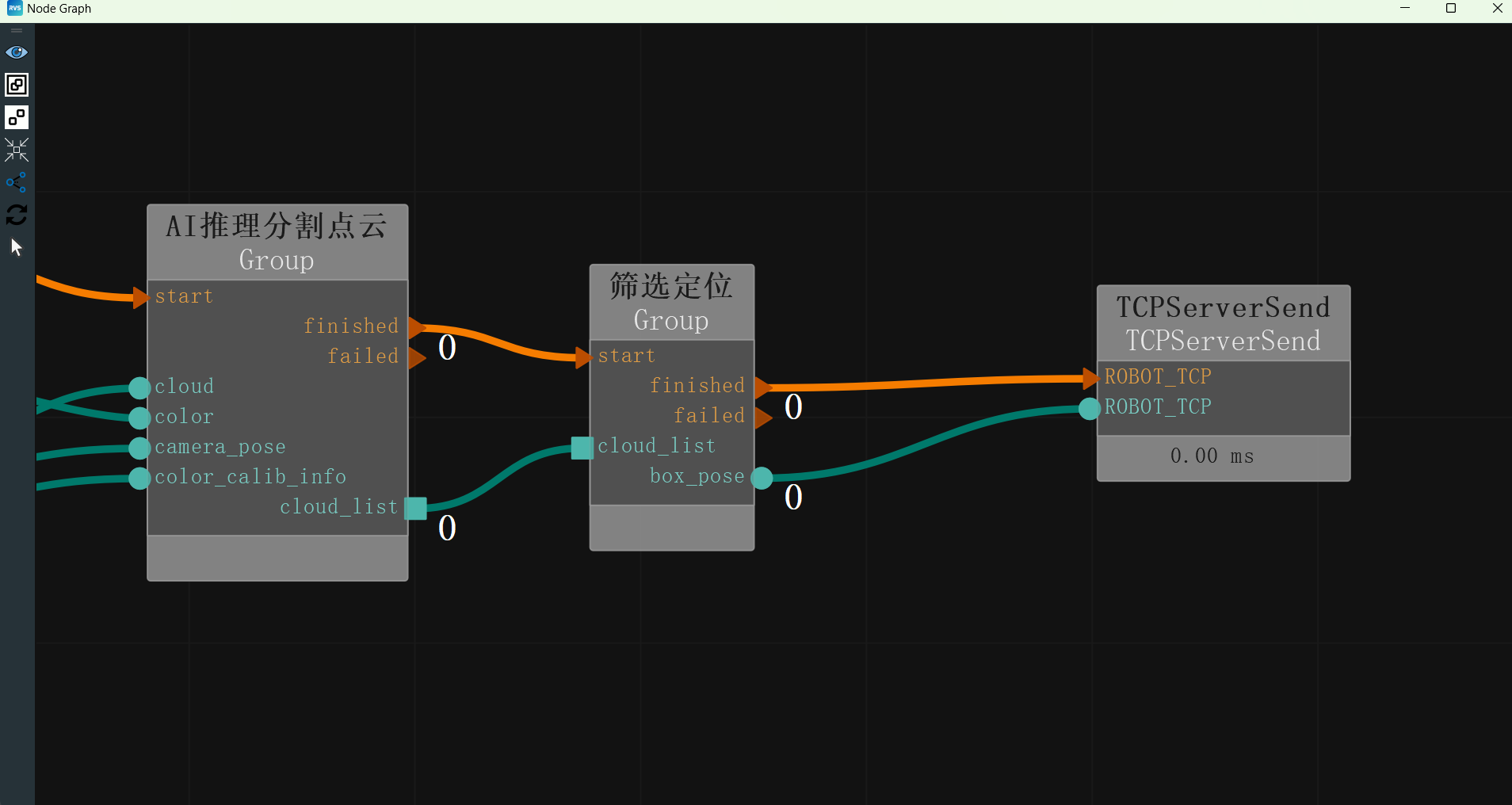
- The node diagram connections are as follows:

Coordinate System Conversion

After loading the data, perform coordinate system conversion to convert the camera intrinsic parameters combined with the hand-eye calibration parameters to the robot coordinate system. This conversion involves camera extrinsic parameters and hand-eye calibration results.

Note

Please refer to the Hand-Eye Calibration Tool online documentation to obtain the actual calibration results. Offline calibration result data is stored in rgb2tcp.txt.

Operation Process

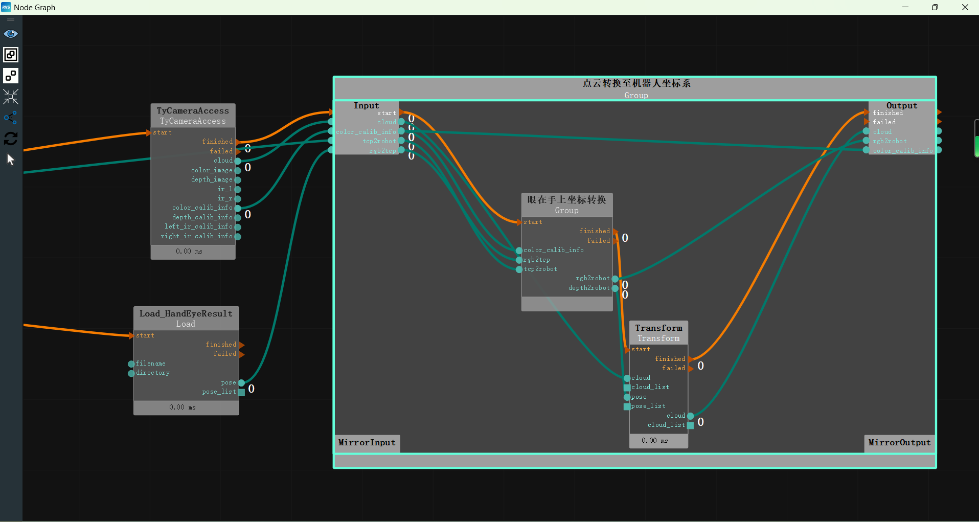
Right-click in the node diagram and select “Create New Group Here” to convert the point cloud to the robot coordinate system.
- Set the new Group parameters:
  - node_name → Point Cloud Conversion to Robot Coordinate System
- Connect node ports:
  - Connect TyCameraAccess's end port to Group's start port
  - Connect TyCameraAccess's point cloud port to Group's Input area
  - Connect Selector_TCP's coordinate port to Group's Input area, right-click Group's internal coordinate port to rename it to tcp2robot
  - Connect Load_HandEyeResult's coordinate port to Group's Input area, right-click Group's internal coordinate port to rename it to rgb2tcp
    
    The node diagram connections are as follows:
Add the EyeInHand coordinate conversion and transform nodes to the Point Cloud Conversion to Robot Coordinate System Group. The EyeInHand coordinate conversion is used to calculate the transformation matrix, and the transform node is used to perform point cloud conversion based on the calculated transformation matrix.
- Set Transform node parameters:
  - Type → Cloud
  - Cloud → Visible → -2
- Connect node ports:
  - Connect Group's start port to EyeInHand coordinate conversion's start port
  - Connect EyeInHand coordinate conversion's end port to Transform's start port
  - Connect Transform's end port to Group's end port
  - Connect Group's point cloud port to Transform's point cloud port
  - Connect Group's color calibration parameter port to EyeInHand coordinate conversion's color calibration parameter port
  - Connect Group's tcp2robot port to EyeInHand coordinate conversion's tcp2robot port
  - Connect Group's rgb2tcp port to EyeInHand coordinate conversion's rgb2tcp port
  - Connect EyeInHand coordinate conversion's depth2robot port to Transform's coordinate port
  - Connect Transform's point cloud port to Group's Output area
  - Connect EyeInHand coordinate conversion's rgb2robot port to Group's Output area
  - Connect Group's color calibration parameter port to Group's Output area
    
    The node diagram connections are as follows. Double-click the Group blank area to collapse it.

AI Inference and Point Cloud Segmentation

In actual work, boxes are often tightly packed, and the upper surface point clouds of multiple boxes may merge into a single large point cloud that is difficult to segment. To address this issue, you can train an AI model and perform AI inference to obtain the box point cloud list.

AI training requires certain configurations. If the configuration requirements are not met, you can directly use the .mask file in the offline data package for inference. The entire process is divided into four main steps: recording, annotation, training, and inference.

Operation Process

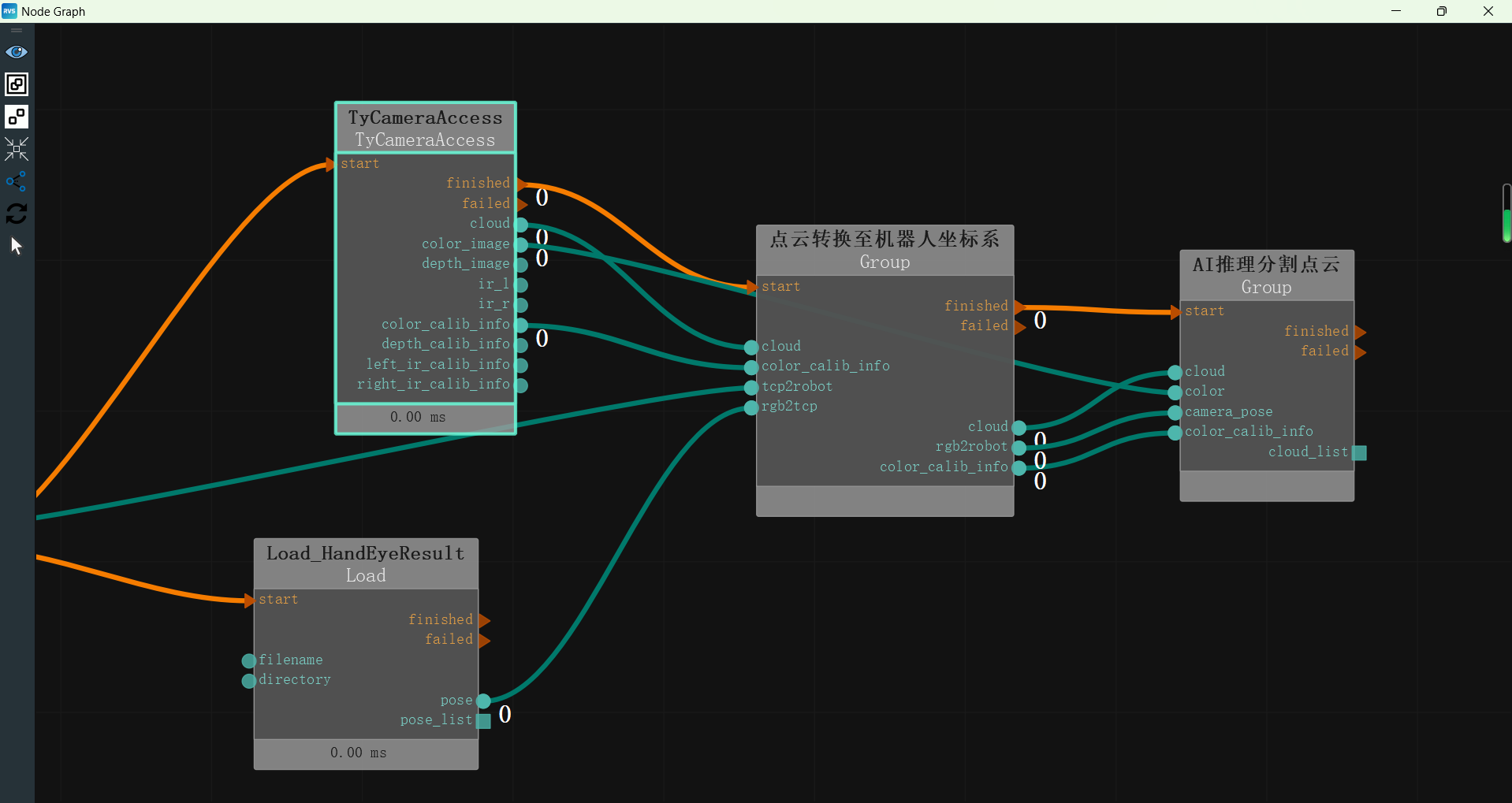
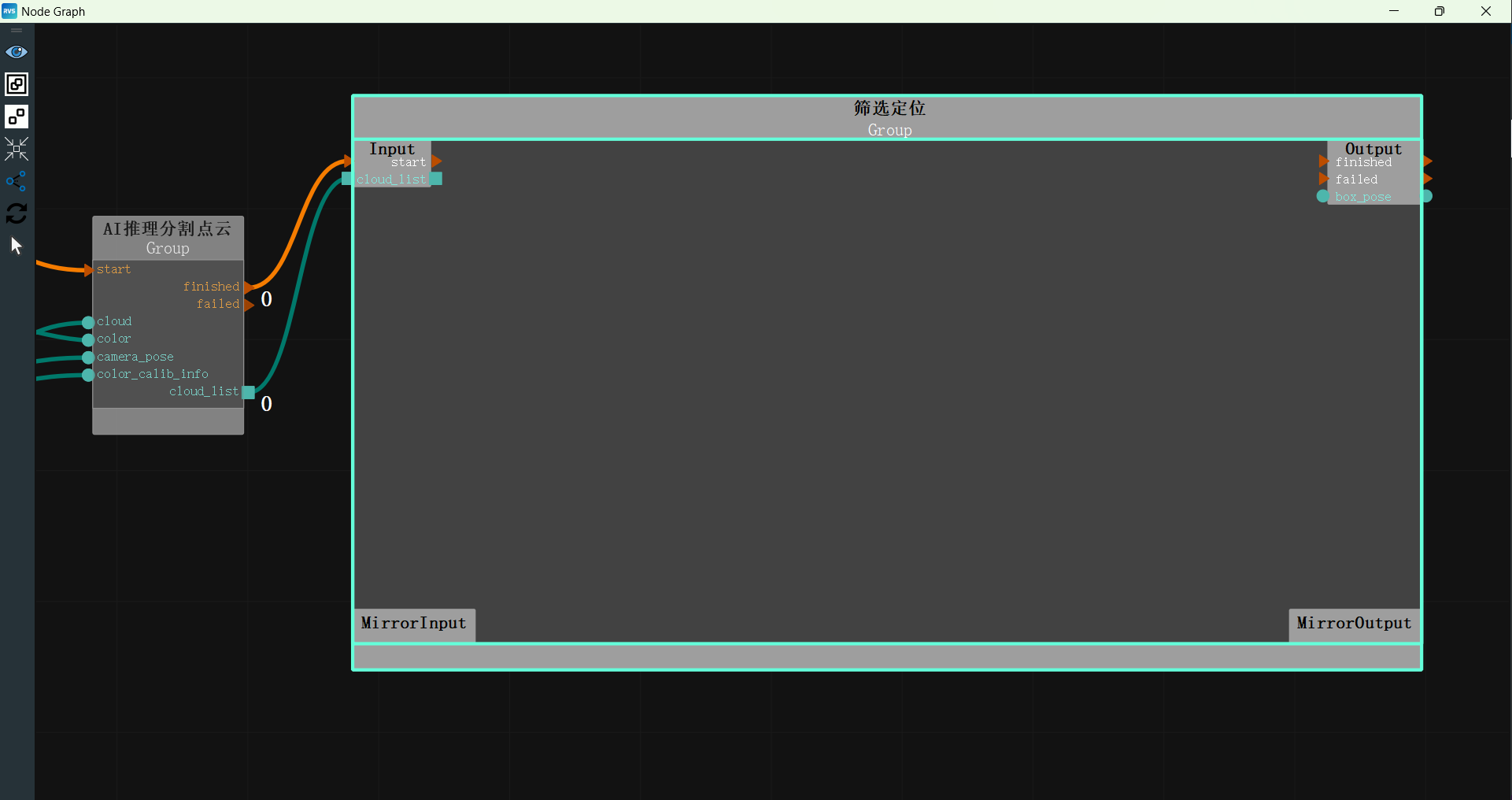
Add the AI Inference Segmentation Point Cloud group to the node diagram to perform color image AI recognition and segment the corresponding recognition area into a point cloud list.
- Connect node ports:
  - Connect Point Cloud Conversion to Robot Coordinate System's end port to AI Inference Segmentation Point Cloud's start port
  - Connect TyCameraAccess node's color image port to AI Inference Segmentation Point Cloud's color image port
  - Connect Point Cloud Conversion to Robot Coordinate System's rgb2robot port to AI Inference Segmentation Point Cloud's camera coordinate port
  - Connect Point Cloud Conversion to Robot Coordinate System's color calibration parameter port to AI Inference Segmentation Point Cloud's color calibration parameter port
    
    The node diagram connections are as follows:
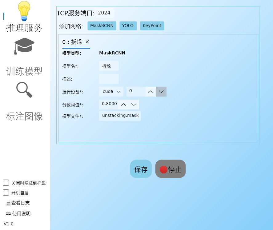
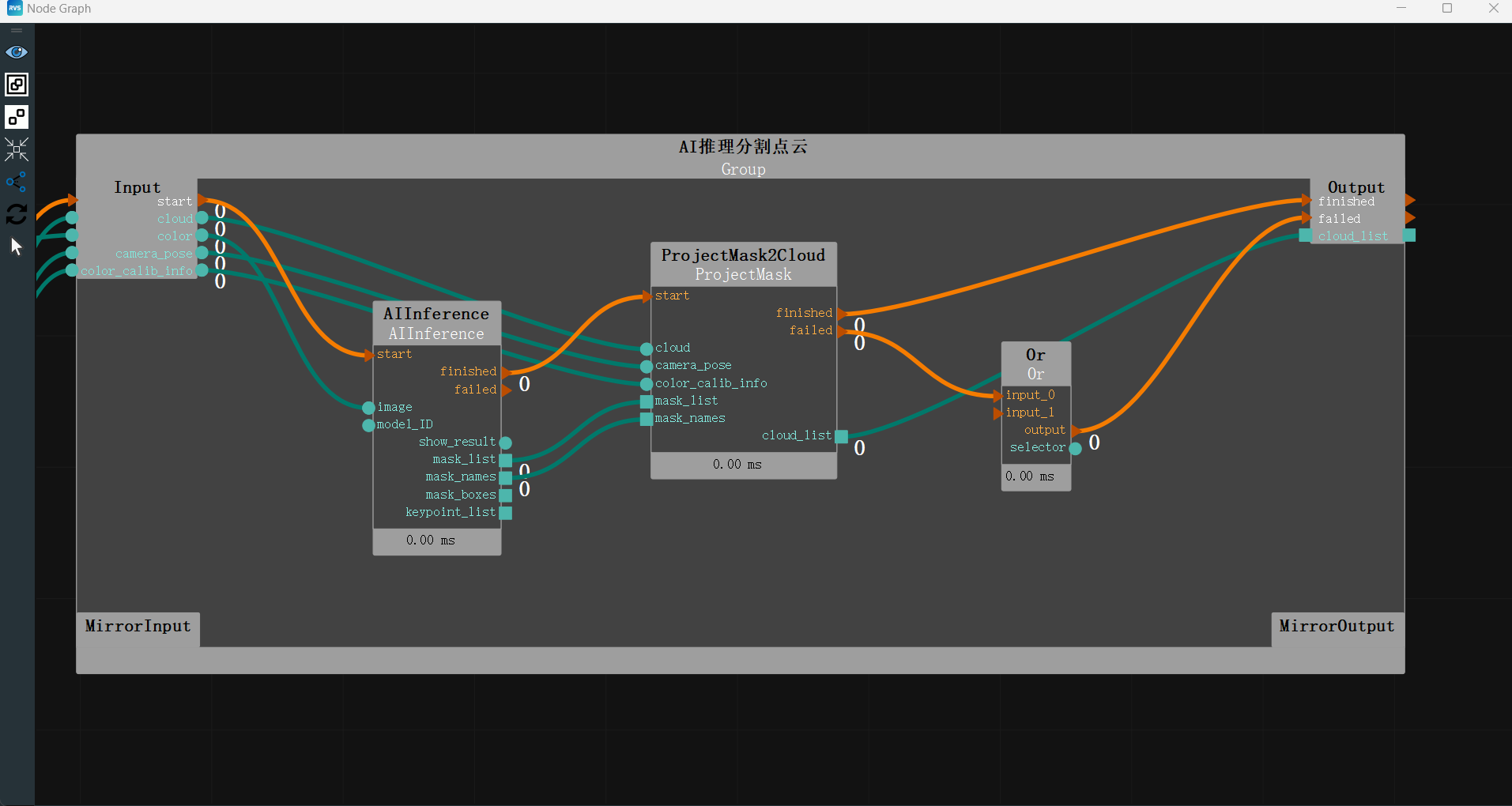
- Set AI Inference Segmentation Point Cloud group’s AI Inference node parameters:
  - Server IP Address → 127.0.0.1
  - Server Port → 2024
  - Model Index → 0
  - Recognition Result Image → Visible
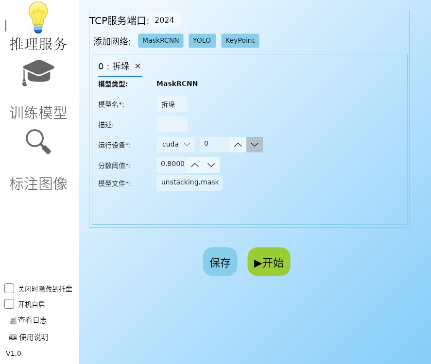
Open RVSAI and enter the Inference Service interface.
- Add the MaskRCNN network and set the parameters:
  - TCP Service Port → 2024
  - Model Name → Unstacking
  - Running Device → cuda 0 (set according to the actual configuration)
  - Score Threshold → 0.8
  - Model File → unstacking.mask

Filtering and Positioning

After obtaining the point cloud list of all detected targets in the robot coordinate system through AI inference, the center coordinates of the point cloud need to be obtained.

Operation Process

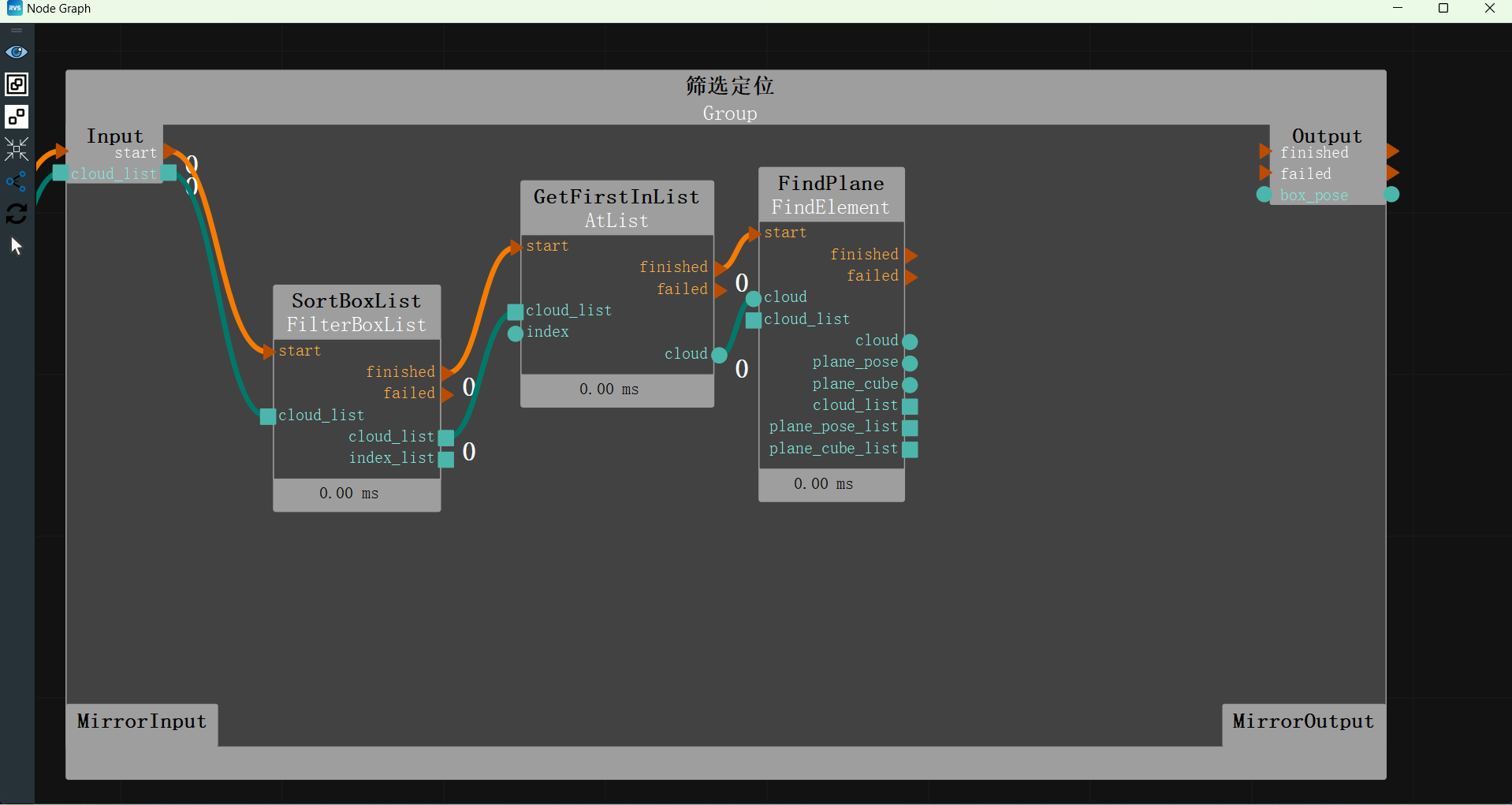
Right-click in the node diagram and select “Create New Group Here” to filter and sort the boxes and then perform positioning.
- Set the new Group parameters:
  - node_name → Filtering and Positioning
- Connect node ports:
  - Connect AI Inference Segmentation Point Cloud's end port to Group's start port
  - Connect AI Inference Segmentation Point Cloud's end port's point cloud list port to Group's Input area
    
    The node diagram connections are as follows:
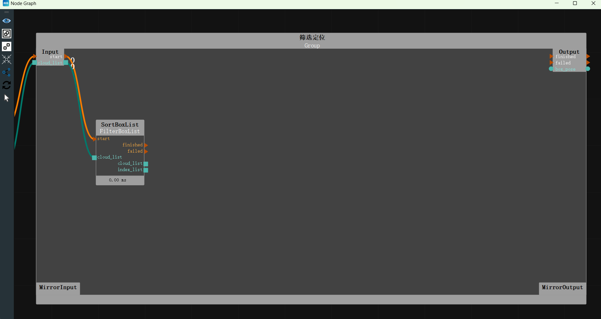
Add the FilterBoxList node to the Filtering Boxes Group to filter the box with the highest Z value and sort the filtered boxes by the Y-axis.
- Set FilterBoxList node parameters:
  - Type → ByAxisZ
  - Selection Mode → Z_MAX
  - Selection Threshold → 0.07
  - X Weight → 0
  - Y Weight → -1
- Connect node ports:
  - Connect Group's start port to FilterBoxList's start port
  - Connect Group's point cloud list port to FilterBoxList's point cloud list port
    
    The node diagram connections are as follows:
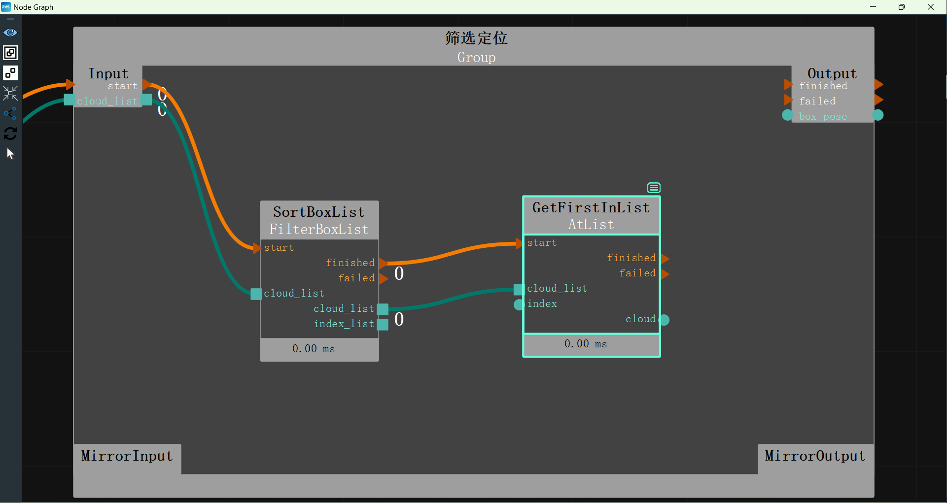
Add the AtList node to the Filtering Boxes Group to extract the first target from the sorted boxes for positioning.
- Set AtList node parameters:
  - node_name → GetFirstInList
  - Type → Point Cloud
  - Mode → Single Index Extraction
  - Index → 0
- Connect node ports:
  - Connect FilterBoxList's end port to GetFirstInList's start port
  - Connect FilterBoxList's point cloud list port to GetFirstInList's point cloud list port
    
    The node diagram connections are as follows:
Add the FindElement node to the Filtering Boxes Group to find the plane in the point cloud.
- Set FindElement node parameters:
  - node_name → FindPlane
  - Type → Plane
  - Distance Threshold → 0.003
- Connect node ports:
  - Connect GetFirstInList's end port to FindPlane's start port
  - Connect GetFirstInList's point cloud port to FindPlane's point cloud port
    
    The node diagram connections are as follows:
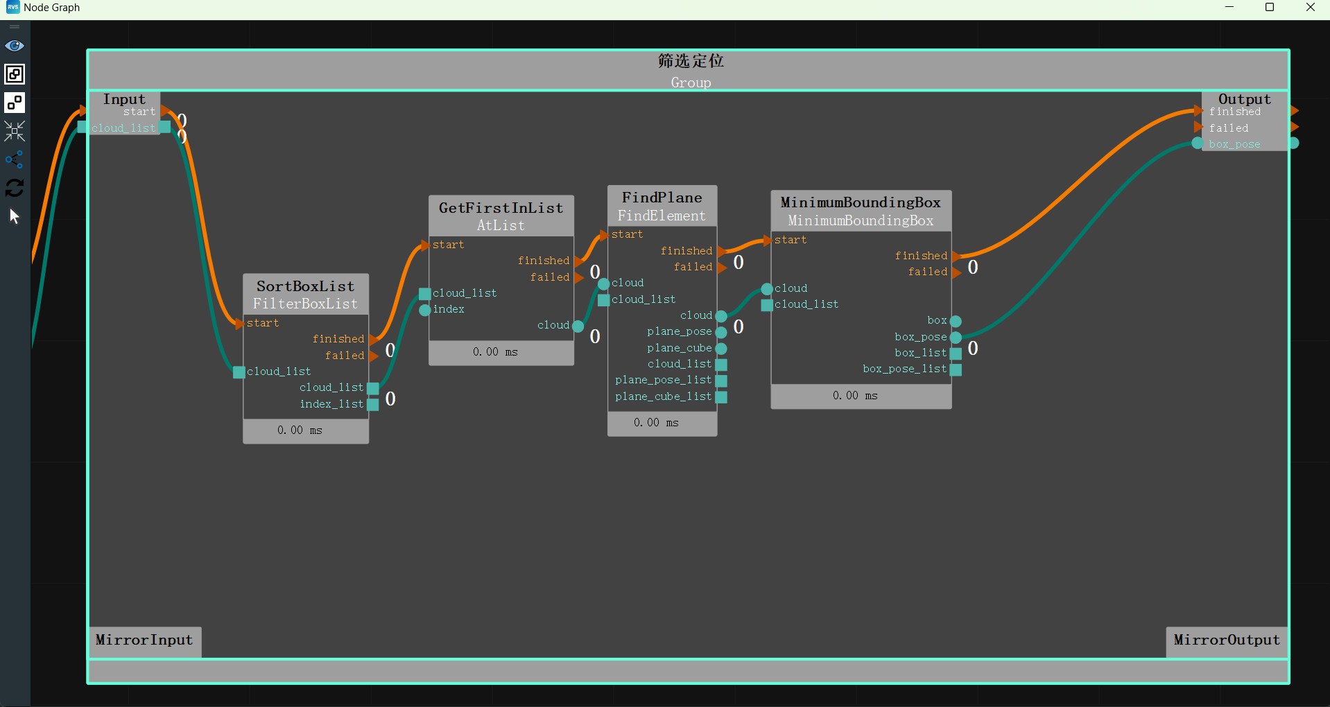
Add the MinimumBoundingBox node to the Filtering Boxes Group to locate the center of the point cloud using the minimum bounding box.
- Set MinimumBoundingBox node parameters:
  - node_name → FindPlane
  - Type → Fast
  - Mode → X > Y > Z
  - Distance Threshold → 0.003
  - Z Axis Direction → World Coordinate System Z Axis Negative Direction
  - X Axis Direction → World Coordinate System X Axis Positive Direction
  - RX Reference Value → 0
- Connect node ports:
  - Connect FindPlane's end port to MinimumBoundingBox's start port
  - Connect FindPlane's point cloud port to MinimumBoundingBox's point cloud port
  - Connect MinimumBoundingBox's end port to Group's end port
  - Connect MinimumBoundingBox's bounding cube center coordinate port to Group's Output area
    
    The node diagram connections are as follows:

Communication Sending

Operation Process

Add the TCPServerSend node to the node diagram to send the located pose to the robot.
- Right-click the TCPServerSend node and open the node panel:
  - Click
  - Port Name → ROBOT_TCP
  - Data Type → Pose
  - Prefix → ROBOT_TCP,
  - Data Separator → ,
  - Suffix → #
    
    The TCPServerReceive node panel configuration is as follows:
    
    Note
    
    The communication string format can be customized. The format in this case is: “ROBOT_TCP,X,Y,Z,RX,RY,RZ#”.
Connect the nodes.
- The node diagram connections are as follows:

Robot Simulation Picking

After completing the above operations, the target point coordinates are obtained. Load the robot model to simulate picking.

Operation Process

Add the SimulatedRobotResource to the Resource Group to load the simulated robot model.
- Set SimulatedRobotResource node parameters:
  - Auto Start → Yes
  - Robot Model File → data/EC66/EC66.rob
  - Tool Model File → data/Tool/EliteRobotSucker2.tool.xml
  - Robot → Visible
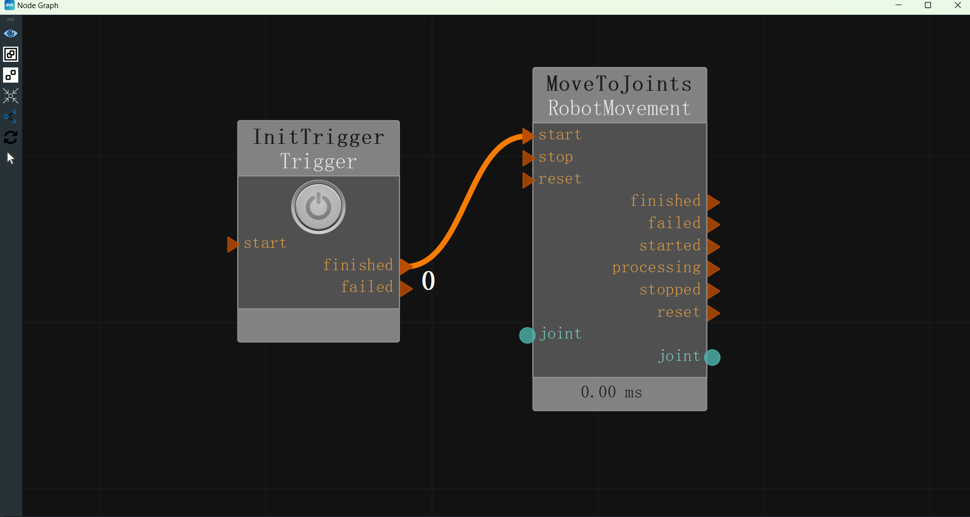
Add the Trigger node to the node diagram to initialize the trigger run.
- Set Trigger node parameters:
  - node_name → InitTrigger
  - Type → Initialization Trigger
Add the RobotMovement node to the node diagram to simulate robot joint movement and move to the initial pose using custom joint values.
- Set RobotMovement node parameters:
  - node_name → MoveToJoints
  - Type → Move Joint
  - Joint → 0 -1.495489955 1.512199998 -1.627550006 1.499660015 -0.04329660162
- Connect node ports.
  - Connect InitTrigger's end port to MoveToJoints's start port
    
    The node connections are as follows:
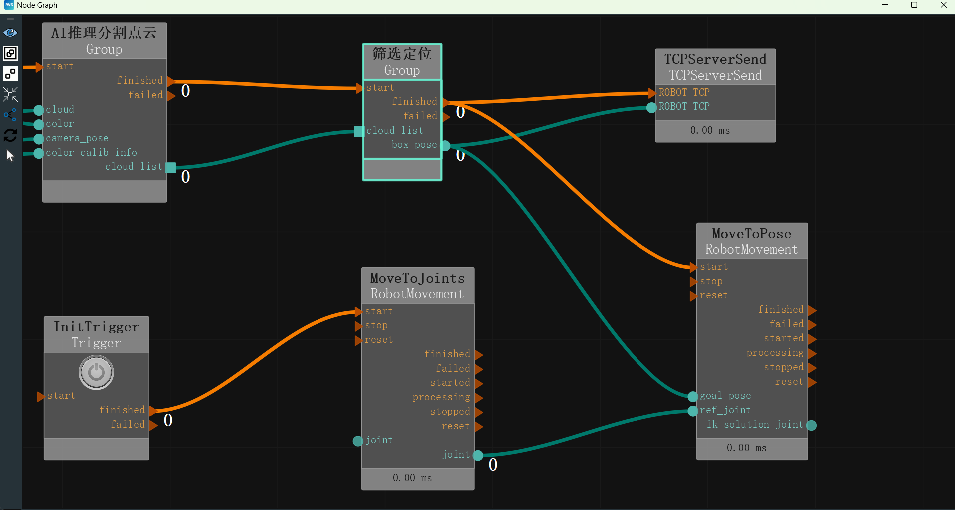
Add the RobotMovement node to the node diagram to simulate robot TCP movement and move the simulated robot based on the located pose.
- Set RobotMovement node parameters:
  - node_name → MoveToPose
  - Type → Move TCP
  - Joint → 0 -1.495489955 1.512199998 -1.627550006 1.499660015 -0.04329660162
  - As Tool Coordinate → Yes
- Connect node ports.
  - Connect Filtering and Positioning's end port to MoveToPose's start port
  - Connect Filtering and Positioning's bounding cube center coordinate port to MoveToPose's goal_pose port
  - Connect MoveToJoints's joint port to MoveToPose's reference joint port
    
    The node diagram connections are as follows:

The complete XML is provided in the unstacking_runtime/unstacking.xml path.

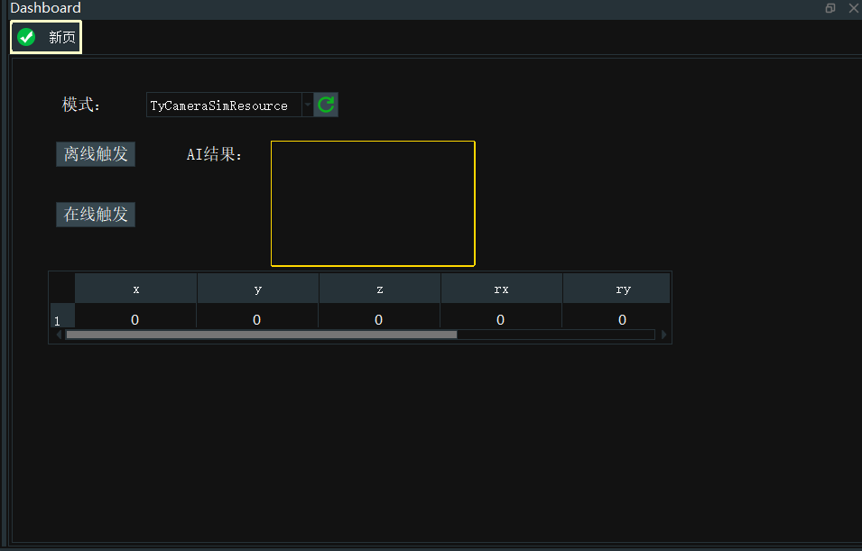
Interaction Panel Creation

The tools in the interaction panel can be bound to the exposure and output of node attributes in the node diagram. Input tools can quickly modify node attribute parameters, and output tools can quickly view node output results.

Edit the interaction panel.
- Right-click the interaction panel and select Unlock. The interaction panel will enter edit mode.
Add input tools Label and Combo Box to the interaction panel.
- Label
  - Double-click “label” and rename it to “Mode:”.
- Combo Box
  - In the node diagram, find the TyCameraAccess node. In the attribute panel, expose the camera resource property .
  - Right-click the Combo Box and select Show Control Panel.
  - In the exposure parameters, select the MainGroup/TyCameraAccess parameter box and click the bind button.
  - Click OK to bind the node parameter to the control.
Add input tools Button (two instances).
- Button
  - Double-click “button” and rename it to “Offline Trigger”.
  - In the node diagram, find the Offline Trigger node. In the attribute panel, expose the trigger property .
  - Right-click the Button and select Show Control Panel.
  - In the exposure parameters, select the MainGroup/Offline Trigger parameter box and click the bind button.
  - Click OK to bind the node parameter to the control.
- Button
  - Double-click “button” and rename it to “Online Trigger”.
  - In the node diagram, find the Online Trigger node. In the attribute panel, expose the trigger property .
  - Right-click the Button and select Show Control Panel.
  - In the exposure parameters, select the MainGroup/Online Trigger parameter box and click the bind button.
  - Click OK to bind the node parameter to the control.
Add input tools Label and output tools 2D Image to the interaction panel.
- Label
  - Double-click “label” and rename it to “AI Result:”.
- 2D Image
  - In the node diagram, find the AI Inference Segmentation Point Cloud. In the attribute panel, enable the show_result_visibility visualization.
  - Right-click the 2D Image and select Show Control Panel.
  - In the exposure parameters, select the MainGroup/AI Inference Segmentation Point Cloud/AIDetect parameter box and click the bind button.
  - Click OK to bind the node parameter to the control.
Add input tools Table to the interaction panel.
- Table
  - In the node diagram, find the MinimumBoundingBox node. In the attribute panel, enable the bounding cube center coordinate visualization .
  - Right-click the Table and select Show Control Panel.
  - In the exposure parameters, select the MainGroup/Filtering and Positioning/MinimumBoundingBox parameter box and click the bind button.
  - Click OK to bind the node parameter to the control.
The interaction panel creation is as follows:

AI Training

This section mainly explains how to collect training images. The complete process is divided into three steps: collection, annotation, and training. For detailed information on annotating training images and training AI models, please refer to the following online documentation: Annotate Training Images and Train AI Model.

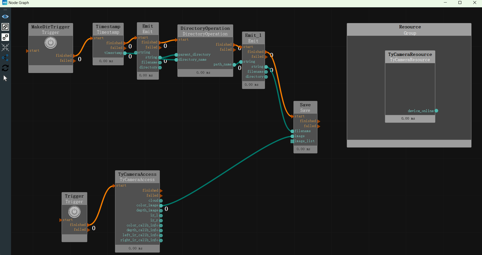
Collect Training Images

Open unstacking_runtime/MaskRCNN/ty_ai_savedata.xml. The content is basically the same as recording RGB images. Here, we only need to adjust the string parameter in Emit to set the desired path. Click the Capture button to record images. Ensure that the number of recorded images is more than 10, the more the better.

When collecting images, we should pay attention to the following points:

Background Lighting
- A single stable light source with appropriate brightness and no excessive reflections.
- Outdoor lighting conditions vary too much and are not recommended.
Consider Complex Working Conditions: Ensure that the sampled data is representative of the actual global sample, not just a special case of the global sample.
- Diversify target objects and avoid using fixed single target objects. If the number of available samples is small, consider using both sides of the sample (if both sides are the same) to double the samples.
- Diversify working conditions. For target objects, consider as many scenarios as possible in which they appear in the working conditions, and capture images in multiple situations:
  - If the project involves different sizes, poses of the stack, and poses of the target in the stack, the training data should cover these diverse situations.
  - Fully consider the deviation margin between the training samples and the actual running samples. For example, if the stack is only placed horizontally, we should also consider adding a small tilt angle to the stack during training, as it is impossible to be perfectly horizontal in practice. Similarly, if the actual operation involves machine placement with targets closely packed, ensure that the targets are closely packed during training data collection, rather than being randomly placed with loose gaps.
  - For a small number of possible target damages or wrinkles, although they rarely occur, if the project requires recognition, specifically collect more damaged targets for data collection. Even if the proportion of damaged targets in the training samples is greater than their actual proportion, this is still meaningful.
Image Quality
- The target edges should be clearly visible to the human eye, especially for the farthest layer of targets from the camera. Otherwise, consider changing the camera. For specific image recording, refer to the rgb images in unstacking_runtime/unstacking_data.

Unstacking Results

As shown below, in the 3D view, the robot end effector accurately points to the center of the recognized object. RVS_result

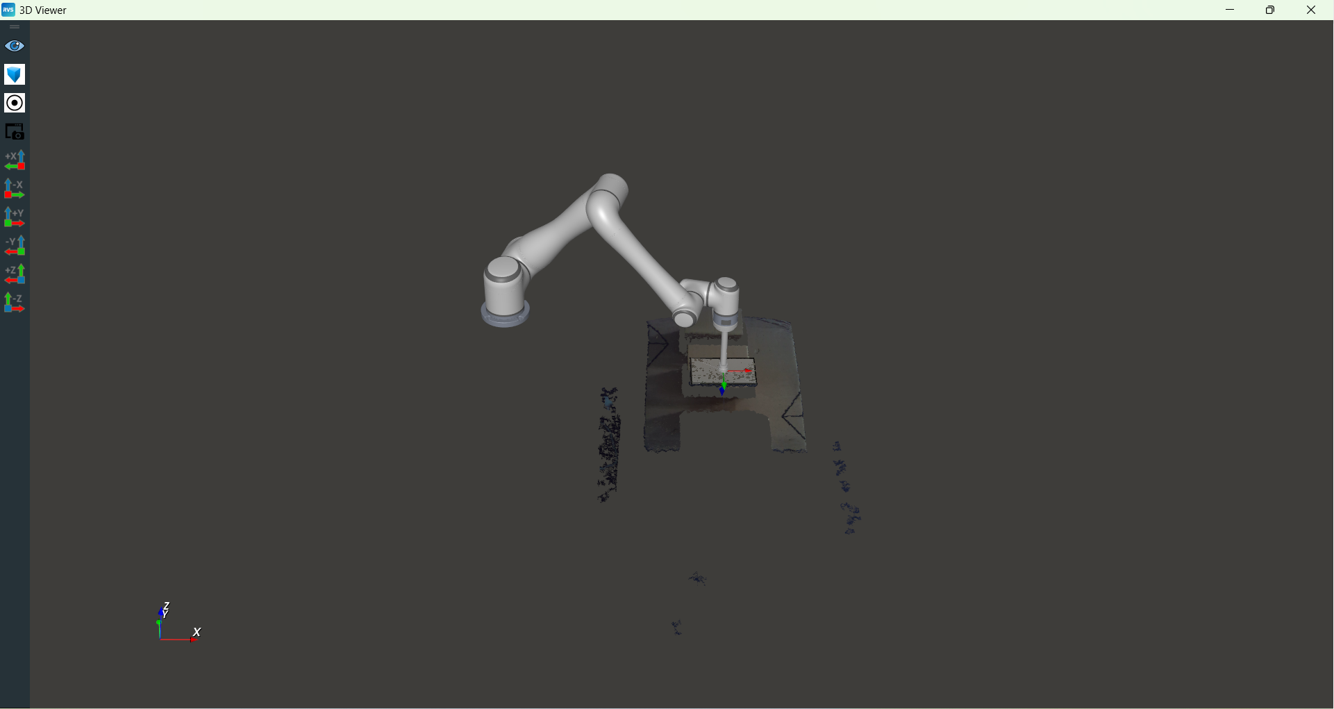
Through the above visualization results, the performance and accuracy of automatic unstacking can be clearly evaluated.