Common function

Image captured by Tuyang camera

Add TyCameraResource

In the menu bar - Resource, add the TyCameraResource resource node to ResourceGroup in the node graph, add the TyCameraAccess node in the search result to the node graph, and adjust the node parameters as required. The default property parameters and parameter descriptions of the TyCameraResource node are as follows.

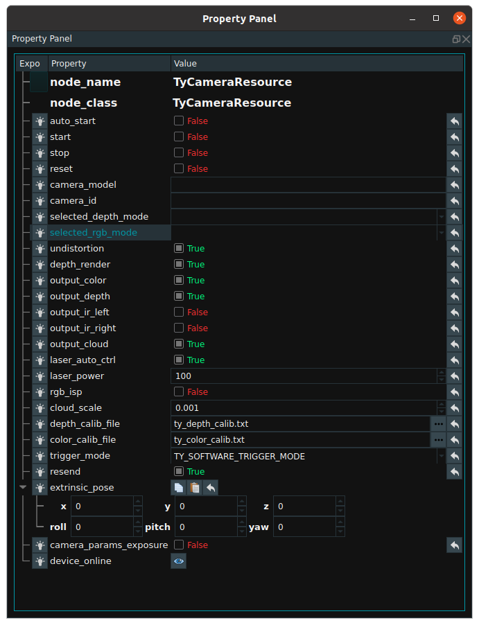
• auto_start：Used to enable the resource node.

  • True：The resource thread is automatically started when the RVS software is running for the first time.

  • False：Resource threads are not automatically started.

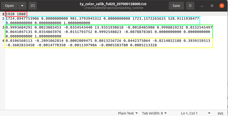
• start / stop：Threads used to enable and disable resource nodes.

• reset：After open the resource thread if need to change the property parameters, need to select this option to reset.

• camera_id：This parameter is not entered by default. After opening the resource thread, it will automatically find all the Tuyang cameras in the network segment where the current industrial computer is located and print the hardware information of these devices in the terminal, and then randomly select a device for link. If you want to specify a Tuyang camera device to be connected, you need to fill in the device’s code to the camera _id option. The code can be viewed on the camera device hardware, or it can be found in the printed information of the above terminal.

• selected_depth_mode/selected_rgb_mode：When connected to the device, the depth map is automatically selected and displayed, as well as the image size of the 2D map, which affects the size of the resulting point cloud image. You can change it later, but you need to set the reset option.

• undistortion：The rgb is dedistorted before output.

• output_***：Used to set whether to output an image. If you want to output a point cloud, you need to check output_depth and output_cloud.

• laser_auto_ctrl：Laser adaptive mode. When false, laser_power can set the intensity of the laser.

• rgb_isp：Preprocessing of rgb images.

• depth_calib_file 与 color_calib_file：The factory calibration parameters of the depth camera and 2D camera stored in the camera device will be automatically read after the resource thread is started and saved to a file according to the file path corresponding to the two parameters. Document content description:

  • color_calib_file:

    • The first line (red area below) indicates the lens resolution used by the camera’s RGB lens for factory calibration. In actual use of the camera, only if the camera resolution is consistent with the values here, you can directly use the following internal parameter matrix. Otherwise, it is necessary to scale the corresponding value (but there will be a certain loss of precision).

    • The second line (blue area below) represents the parameters for the camera’s RGB lens. There are 9 values in total, and it is a 3 by 3 matrix arranged in rows. The matrix form is [fx,0,cx,0,fy,cy,0,0,1], where fx represents the focal length of the camera in the X-axis direction (in pixels), and cx represents the center of the camera in the X-axis direction (in pixels); fy and cy are similar.

    • The third line (green area below) represents the external parameter of the camera’s RGB lens, which is the spatial coordinate transformation matrix from the RGB lens to the left IR lens. There are 16 values in total, and it is a 4 * 4 matrix arranged in rows. The 3 * 3 module in the upper left corner represents rotation, and the 1 * 3 in the upper right corner represents translation. Translation values are measured in millimeters.

    • The fourth line (yellow area below) represents the distortion parameters of the camera’s RGB lens, with a total of 12 values. It can be used to perform distortion correction on raw RGB images.

      Notes：For depth_calib_file, the description remains the same as above. In particular, since the depth camera is a virtual camera, its distortion parameters and external parameters are zero matrices.

• trigger_mode：

  • TY_SOFTWARE_TRIGGER_MODE：For the software trigger mode, the camera captures one frame of image each time the trigger command is sent.

  • TY_HARDWARE_TRIGGER_MODE：The hardware trigger mode is used to capture data by the hardware trigger camera.

  • TY_TRIGGER_MODE_OFF：The camera keeps capturing images, and each time the trigger command is sent, the camera sends back a frame of data to RVS. TY_TRIGGER_MODE_OFF is more efficient in terms of time, but please note that the image obtained by sending trigger at time t is not collected at time t, but at time T-T0. t0 depends on the camera model and is generally larger than 0.5 seconds.

• resend：

  • True：It is resold every time the camera sends back RVS data and a packet loss occurs.

  • False：Packet loss is not resold every time the camera sends back RVS data.

• extrinsic_pose：It cannot be modified. After loading from the current camera resource, read the external parameter of the current camera’s rgb camera from the sdk (that is, the conversion matrix of the rgb camera to the left ir depth camera) and convert it into pose form for display.

• camera_pararms_exposure：Whether to expose some of the camera’s functional property parameters.

Add the Tuyang camera collector

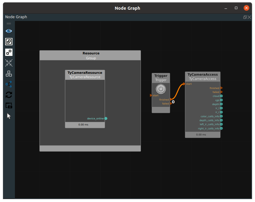
Step 2：Add the trigger and TyCameraAccess nodes to the node graph and connect the finished port to the start port of the TyCameraAccess node.

Camera data acquisition in real time

Step 3 :

1. Click the Run button in the toolbar at the top of the RVS software.

2. Click on TyCameraResource and check the Start Automatically or Start property.

3. Select the trigger property in the property bar of the trigger node, and the output_? Selected by the TyCameraResource node will be displayed. If the collected data needs to be displayed, the visual properties in the property bar of the TyCameraAccess node need to be changed. If the loop attribute of the trigger node is checked, the image will be continuously captured.

The node graph is connected as follows.

Saving data

RVS software provides Save node to Save the data. Select the type attribute as required. The following uses type as Image as an example.

Enter the file path in the filename port on the left of the Save node (or in the filename attribute of the node), and enter the port (or image_list port) on the left image to enter the image, trigger the start port of the node, you can save the image to the local.

Notes：If both the filename attribute of the node and the filename port to the left of the node are assigned a value, the value of the filename port to the left of the node is preferred.

Save—Image：

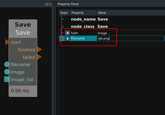
In addition, there are PointCloud, Pose, JointArray, String, Cube and other types. Directly enter the keyword save in the search box of the node list and select the corresponding type attribute.

Reading of local data

RVS software also provides (Load)(http://doc.percipio.xyz/rvs/latest/basic/Load.html) node to read local data. The type attribute includes Cube, Image, JointArray, Line, Path, PointCloud, PolyData, Pose, Shpere, Voxels.

The following uses Image as an example.

The Load node can read a single image or all images in a folder. To read a single image, you need to enter “image path + name” in the filename port on the left side of the node (or in the filename attribute in the property panel). When start is triggered, the image data read will be output to the image port on the right. To read multiple images, you need to enter “image path” in the directory port on the left side of the node (or in the directory property of the properties panel). When the start is triggered, all image data read will be output to the imagelist port on the right in the form of a list.

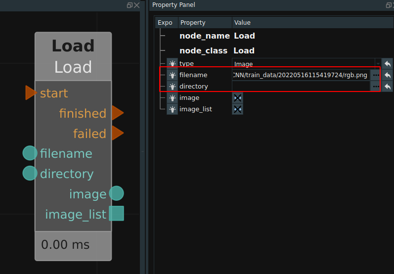
For other type types, select the corresponding type attribute in the save node.

TCP communication

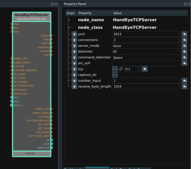
RVS provides a standard TCP node: HandEyeTCPServer, used for RVS program with robot or other communication between industrial control process. The node runs a new thread at the bottom of the RVS program to create and maintain a TCP server side.

Its properties are shown in the following figure.

Pointcloud filtering

DownSampling

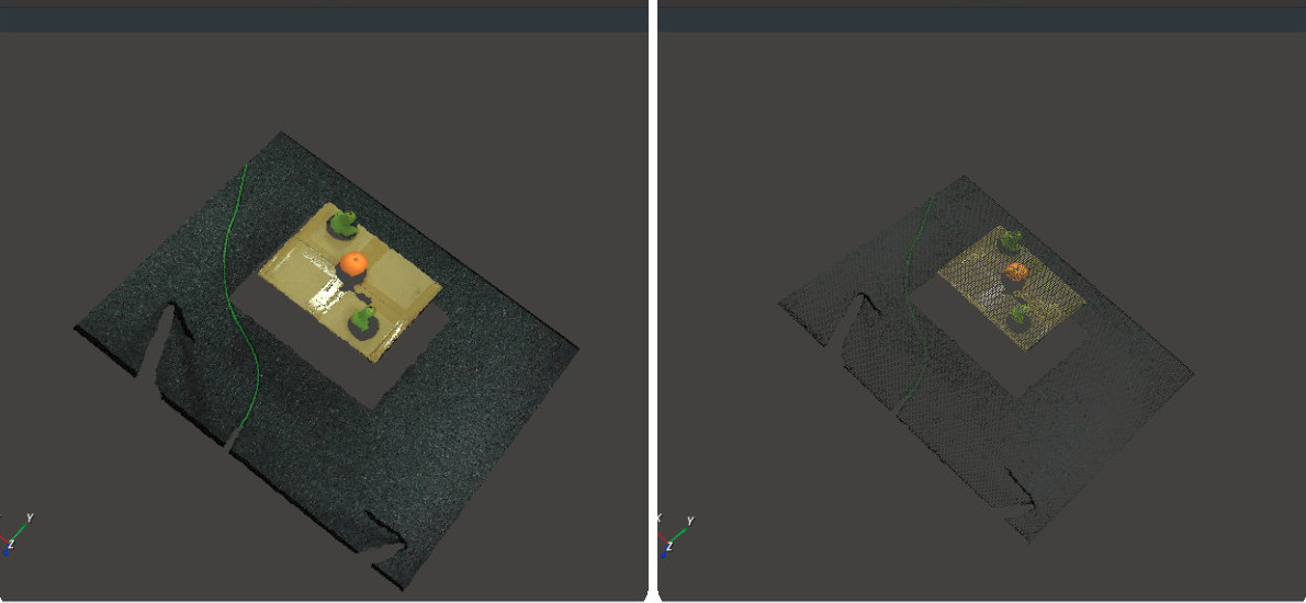
Namely DownSampling node, the role of point cloud is sparse. For some nodes, a small number of sparse point clouds is sufficient to complete the calculation, while too dense point clouds will only reduce the node execution efficiency. In this case, the original point cloud can be considered to perform downsampling and sparse processing before subsequent operations. The following is an example of a connection of the DownSampling node.

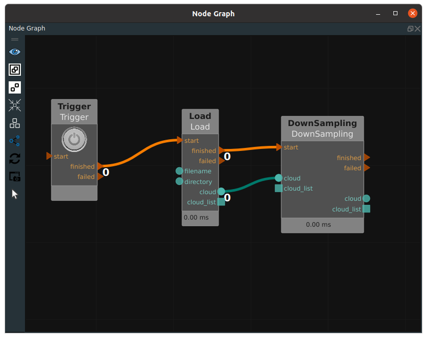
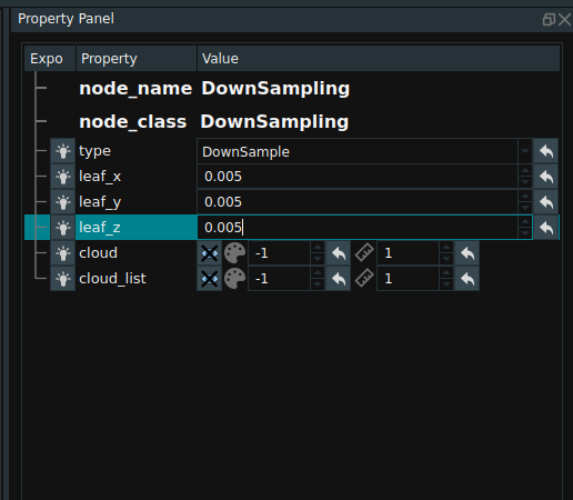
To modify leaf_x, leaf_y, and leaf_z in the node property panel, you can specify the point cloud resampling interval in the xyz axis direction, which is specified as 0.005m, indicating that only one point is taken within the spatial scale of 0.005m * 0.005m * 0.005m.

The picture below shows the pointcloud before and after filtering.

Point filtering

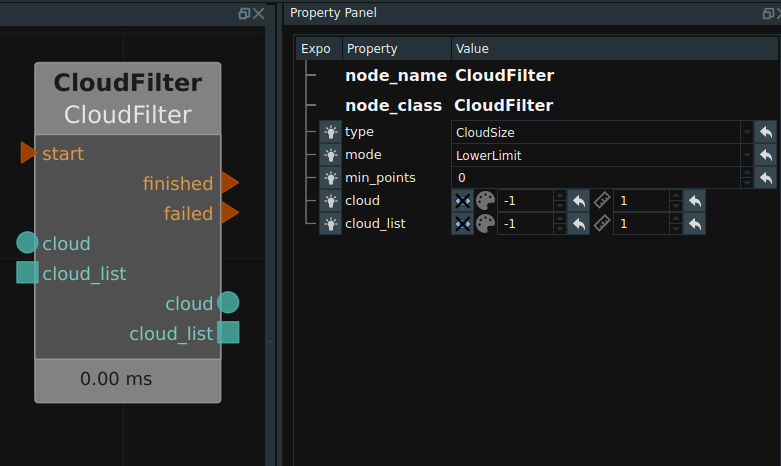
The CloudFilter node, the input point cloud can be points of judgment. You can modify the attribute mode of CloudFilter, which indicates the point cloud filtering method.

Property Minimum and maximum point values that specify the threshold for entered point cloud points. When the mode is combined with the number of points, finished is triggered. Otherwise, failed is triggered.

Plane filtering

FindElement node, can automatically find the corresponding geometric shapes of point cloud, and point to plane according to the distance threshold to filter the point cloud. The type attribute includes Plane, Cylinder, Sphere, Circle, and Line. A connection example is shown in the following figure.

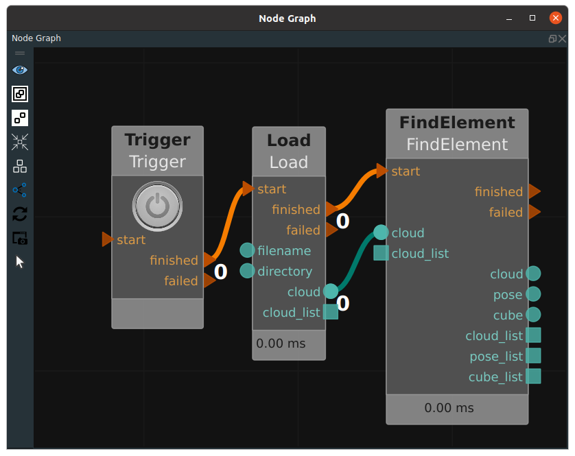
The property pannel is shown below.

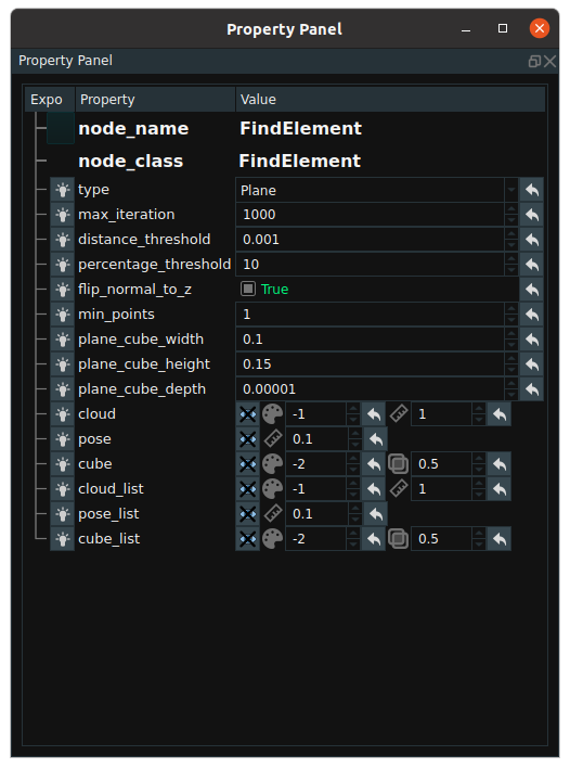
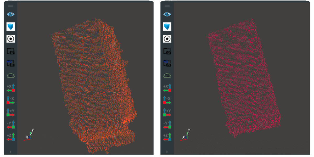
The distance threshold of point cloud filtering can be adjusted by modifying the attribute distance threshold. The following figure respectively shows the output of the original point cloud and the point cloud after finding the plane.

CloudSegment

That CloudSegment node, the type attribute contains: CropboxSegment, PlaneSegment, PassthroughSegment, DiffSegment, NNPDSegment.

The CropboxSegment cuts the point cloud according to the input cube region and needs to be used in conjunction with the Emit-Cube node. An example is shown in the following figure.

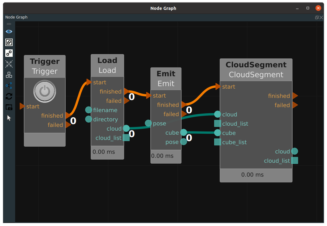
You can cut out the desired point cloud area by adjusting the position and size of the Cube in the 3D view. The image on the right shows the cut out point cloud.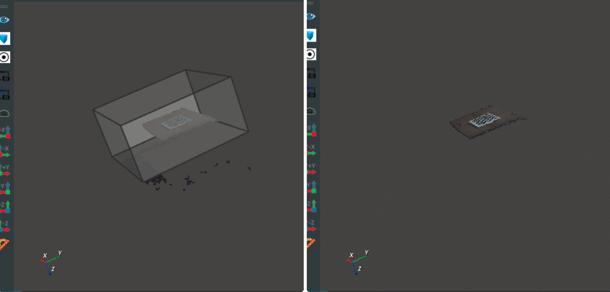

Target location

Position the target’s upper surface attitude

That MinimumBounddingBox node, its effect is according to the target table pastry surrounded by cloud point cloud to obtain the smallest cube box. It is often used for attitude positioning of objects such as bags and bags.

Notes：Since the target is the minimum rectangular bounding box of the surface point cloud, PlaneFinder node processing is often required for the point cloud before the MinimumBounddingBox node calculation, in order to remove the point cloud on the side of the target.

After finding the smallest cube of the target, the node will take the center of the cube as the center of the output attitude, and the direction of the three axes of the cube, ight-width -Depth, as the direction of the three axes of the output attitude, XYZ.

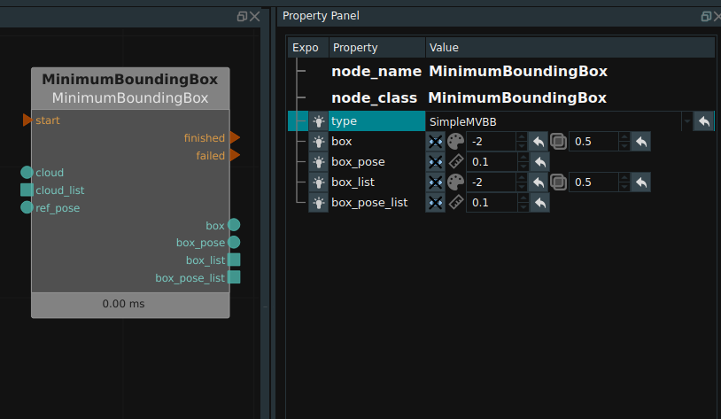
There is a ref_pose data port in the image above. When ref_pose is connected, the resulting Cube will match the Hight - Width - Depth with X, Y and Z by referring to the pose entered in the ref_pose port on the left side of the node. If the port is not connected to data, the ight - Width-Depth default matches X, Y, and Z in Pose(0,0,0,0,0,0).

The effect of node positioning is as follows.

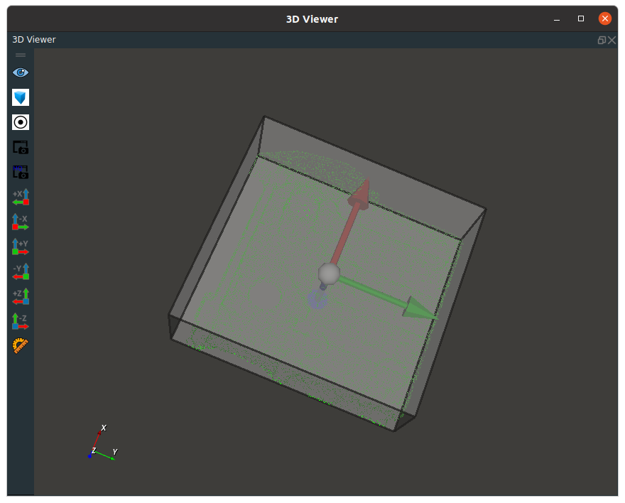
Positioning of center

CloudProcess, the type attribute for CloudCentroid node, is used to enter a point cloud, the output of the coordinates of the point cloud center.

Note:The attitude of the output is automatically selected as the base coordinate system and not along the length and width direction of the target.

Connection examples and effects are shown below.

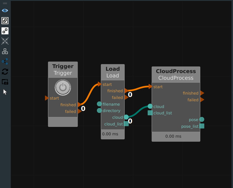
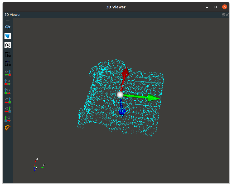
Point cloud clustering

The ClusterExtraction node. According to the set minimum distance parameter tolerance value (as shown in the attribute diagram below), the two target points with a distance greater than this distance are classified into two categories, and the point clouds with a distance smaller than this distance are classified into one category, and finally multiple target point clouds are separated from each other. In addition, the node also limits the minimum and maximum number of point clouds for each point cloud category of the class.

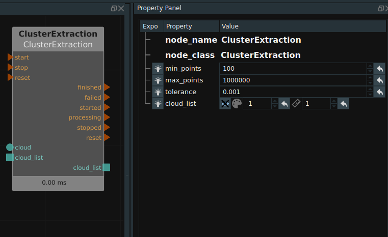
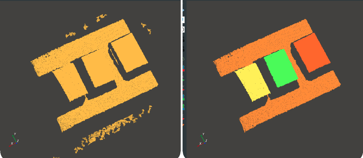
When using this node, the tolerance node should be adjusted as needed. The following two figures respectively show the comparison before and after clustering. (Each color corresponds to a category)

Coordinate system description and attitude transformation

Coordinate system specification

RVS software has a built-in 3D view display environment, the display coordinate system is world coordinate system BaseXYZ, the coordinate origin (0,0,0). The pose we generate through nodes such as Emium-Pose is all based on the BaseXYZ coordinate system.

Our simulation robot is defined by the digital-analog file. The robot has its own base coordinate system RobotXYZ, because we always align the base coordinate system of the robot with the world coordinate system of the production software when making the digital-analog robot. So after importing the analog files in RVS software, RobotXYZ is aligned with BaseXYZ by default.

The 3D point cloud image of Tuyen camera also has its own coordinate system, the left IR coordinate system of the camera CameraXYZ. When we display CameraXYZ in BaseXYZ, the left IR of the camera is placed in the Pose of (0,0,0,0,0,0) by default, so CameraXYZ and BaseXYZ are in the same coordinate system. However, such display is actually meaningless. We need to find the space attitude pose_true of the camera in the robot coordinate system, and then correct the CameraXYZ coordinate system in BaseXYZ according to this attitude.

In addition, the object of our camera, such as the box, has its own object coordinate system ObjXYZ . The body coordinate system is the pose of the target.

Each Pose(x,y,z,rx,ry,rz) in the RVS software represents both an attitude and a 4*4 coordinate transformation matrix, where xyz represents the translation of the matrix and rx/ry/rz represents the rotation of the matrix.

Coordinate transformation

The Transform node, attribute type as a pose, sample as below.

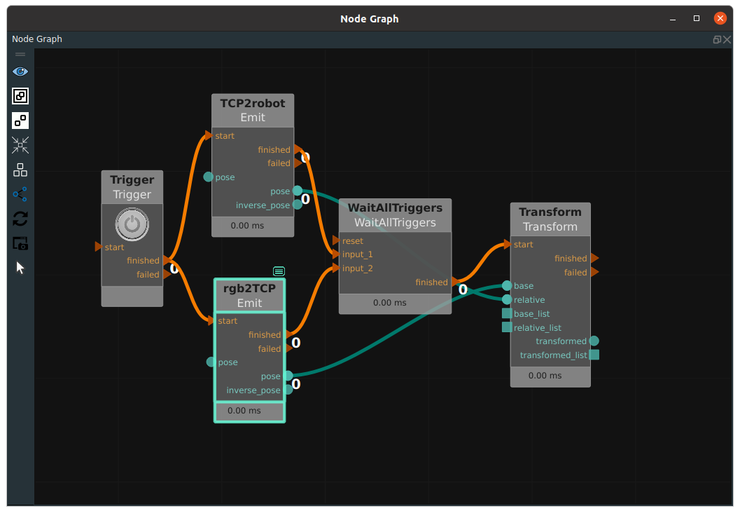
Emit (TCP2robot) in the figure is the pose (or conversion matrix) of the robot flange in the robot coordinate system. Emit (rgb2TCP) is the result of hand-eye calibration, representing the seated conversion matrix from the rgb coordinate system of the camera to the robot flange coordinate system. The former is connected to the left relative port of the Transform node, and the latter is connected to the left base port of the Transform node, indicating that the former matrix is multiplied by the latter matrix, and then the conversion matrix from the rgb coordinate system of the camera to the robot coordinate system can be obtained. Output as pose to the transformed port to the right of the Transform node.

In addition, the Emit nodes in the figure above (TCP2robot and rgb2TCP) have not only a pose port output, but also an inverse_pose port output, which represents the inverse matrix of the former.

Transformation of units

Units that Pose from m/mm, switching between Angle/radian, corresponding to the node for ScalePose. Set itsXYZ ratio: 0.001 to switch from meters to millimeters. Set its’ RPY ratio: 0.01745329 to switch the Angle to radians. Similarly, you can switch backwards.

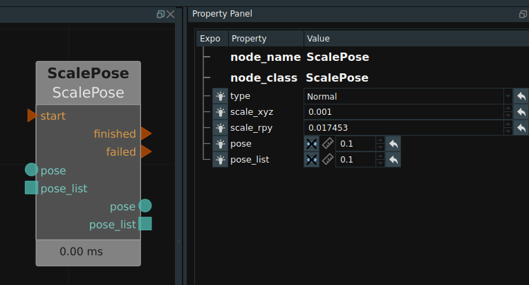
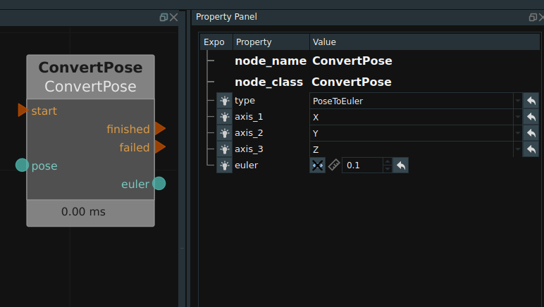
The default rotation mode of Pose rotates the unfixed axis around the Z-Y-X order, can be switched to Euler Angle (rotates the fixed axis around the X-Y-Z order), Corresponding node for ConvertPose operator, the type attribute for EulerToPose and PoseToEuler.

AI module

RVS software is embedded with the cutting-edge CNN deep learning module, which can detect and segment rgb images. We provide nodes for data training and recognition.

AITrain

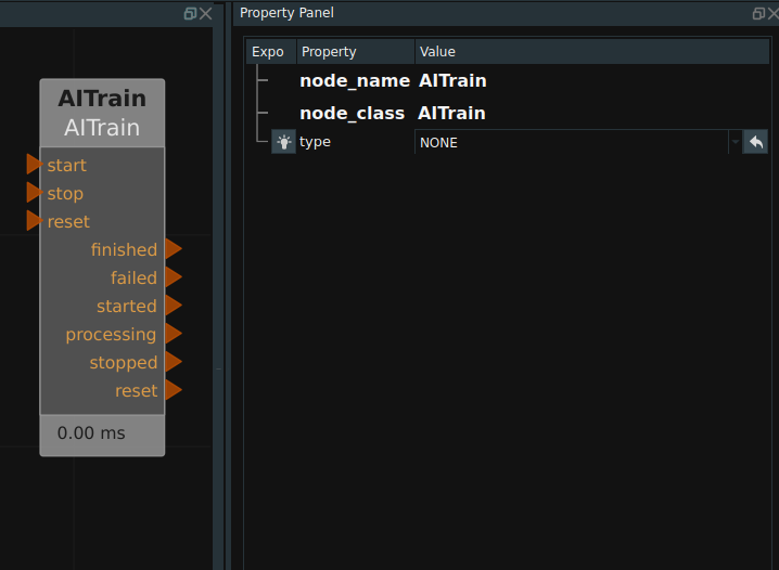
Training data set is required before the preparation, the specific operation in automatic open chock - training AI modules.

When labeling the training data of the RotatedYOLO network, if the target is a rectangular target such as a box, it is recommended that each target be labeled with only four points. If it is a polygon target, you can label as many points as you like (in practice, the algorithm automatically generates a four-point rotating rectangle based on the labels).

Notes：For RotatedYOLO, be sure to use at least two classes of data when training, as single-class training is less effective. If there is really only one category of data, it is recommended to add an additional data that is not used by the current project to train together.

In addition, in order to ensure the training effect, the number of objects in each class should not be less than 200 targets (there are usually multiple targets in a picture).

When annotating training data of KeyPoint network, there are two types of annotation objects.

1. The object itself is marked. The annotation tool of “Polygon/PolyRect” is selected in Labelme software during the annotation, and each annotation point must follow the outline of the object, and the annotation method at this time is equivalent to the data annotation of MaskRCNN network.

2. It refers to the annotation of key points within the target. The annotation tool of “Point/Point” is selected during the annotation in Labelme software, and the location of key points must be within the target. For example, our tagging object is a table, the key point of the design is the table corner, and a quadrilateral area has been marked for the table, then the tagging point must be inside the quadrilateral area marked by the table, not on the border, not outside the border. If the marking areas of multiple targets overlap, such as marking the box and the bar code area above the box at the same time, the key points of our design are not allowed to be marked in the bar code area of the box, because the bar code area is an overlapping area.

When the AITrain node is actually executed, it will automatically format and train the annotated data set. At present, RVS supports three types of neural networks, namely MaskRCNN, KeyPoint, and RotatedYOLO.

Before running it, you need to manually create a category label file with a name ending in “.txt “.

For MaskRCNN and RotatedYOLO networks, each category has a separate line in the category tag file, such as: apple banana pear

The preceding category names apple, banana, and pear are the actual category names defined during data annotation. No Spaces are allowed in the name of each row.

For KeyPoint networks, each line in the category tag file can also contain a corresponding key name. Such as: pear banana top bottom orange

“top” and “bottom” after a banana indicate that two key points are set for a banana type of goal.

After creating the above file, enter the file as the classnames_filepath attribute of the AITrain node. The folder where the marked training data resides is entered as the data_directory attribute of the node.

This node is used for the training of neural networks, and a folder train_output is automatically generated after the training is completed. For the RotatedYOLO network, box_loss generally needs to be reduced to less than 0.03 after the training to achieve a better training effect, and the train_output folder will be automatically created in the used_data/directory after the training is completed. It contains the trained weight file:

used_data

• train_output

  • weights

  • best.pt

  • last.pt

In train_output folder, a part of image data will be randomly selected for inference test based on the last best.pt and the results will be saved as image files. Among them, val_batch? _ labels.jpg is the original labeled data. The corresponding val_batch?_pred.jpg is inference data from which you can get a rough look at the training effects.

Refer to the AITrain node description for more detailed node properties.

AIDetectGPU

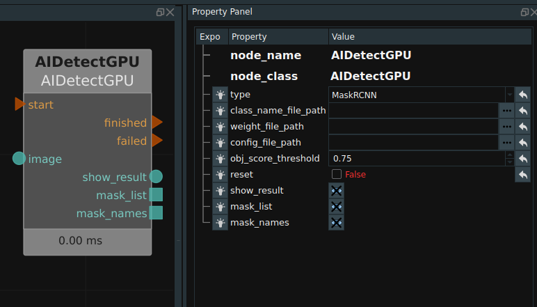
This node can invoke the training results of AITrain node under MaskRCNN and KeyPoint network to conduct a reasoning on an input image, and then obtain the result of object detection or instance segmentation.

The MaskRCNNGPU can be started multiple times in the same RVS. To use this node, you must install a separate nvidia graphics card with at least 4G video memory.

After inference is complete, the inference mask of the target is output to the obj_list output port in the form of a list of images, where each image corresponds to a mask map of the detection target. The length and width of the mask map are consistent with the original image, and it is a grayscale map, the background grayscale is 0, and the location area of the detection target is filled with grayscale 255.

AIDetectGPU node in addition to the output mask map list and the result display diagram, will also output all the inference results of the class name, are output in the form of list, the serial number inside corresponds to one by one. In addition, for the KeyPoint network, an additional list of key points contained in each target is given.

class_name_file_path : For MaskRCNN networks, you can directly use the class name file used during training, that is, txt as the file suffix (or names as the file name suffix), but for RVS1.3 and older versions of the training method, You can also select the series.json file generated during the training data transformation as the named file. For the KeyPoint network, only the annotations.json file generated during the training process can be selected as the named file.

weight_file_path : For RVS1.3 and older training methods, this property should not enter any parameters. For the existing training style, enter the train_output/config.yaml file generated during the training in this property.

See the AIDetectGPU node description document for a more detailed description of node properties.

AIDetectCPU

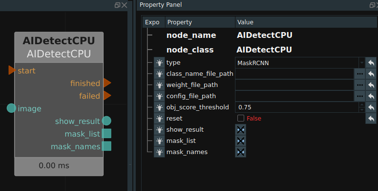
This node is suitable for pure cpu machine inference use without nvidia graphics card. The parameter is the same with AIDetectGPU.

See the AIDetectCPU node description document for a more detailed description of node properties.

RotatedYOLO

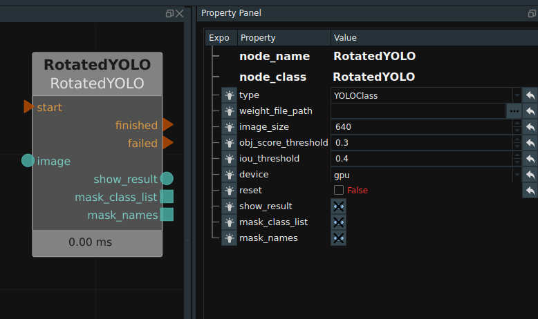
This node can invoke the training results of AITrain node under the RotatedYOLO network to conduct a reasoning for an input image and then obtain the target detection result. This node can start more than one in the same RVS. This node supports both GPU and CPU modes. To use this node’s GPU mode, you must install nvidia’s independent graphics card.

The RotatedYOLO deep learning module and the AIDetectGPU/AIDetectCPU inference node are not mutually exclusive with each other, nor are they mutually exclusive with the python node, and both can run multiple times in the same RVS software.

Due to the relatively simple RotatedYOLO model, the inference speed is faster, but correspondingly, the annotation data required for its training convergence will be much larger than MaskRCNN, and the duration of each training is often greater than 3 hours, and the final target inference precision will be deficient compared with MaskRCNN.

Refer to the RotatedYOLO node specification document for a more detailed description of node properties.

ProjectMask

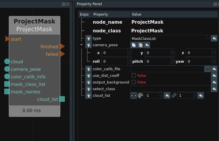
The ProjectMask node can convert the rgb target segmentation results of the AI node into the point cloud image, and then generate multiple target point cloud lists cloudlist.Refer to the ProjectMask node description document for detailed description of node properties.

ProjectPoints

The ProjectPoints node can convert pixels in an rgb image to 3D points in a point cloud (presented in Pose form), and then generate a series of Poselists.

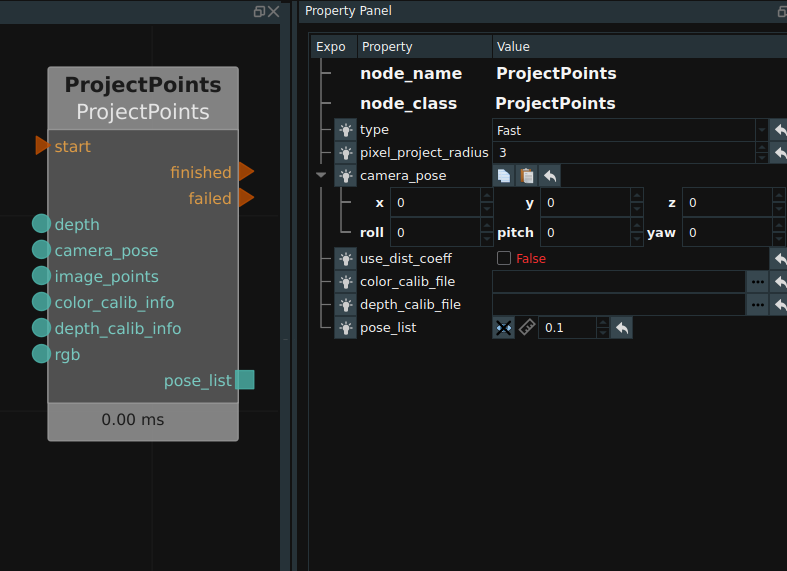
Refer to the ProjectPoints node description document for more detailed descriptions of node properties.

Robot simulation

SimulatedRobotResource

RVS software has created simulation models for many common robots at home and abroad, the file format is “*.rob”, and the library of digital models is still expanding and updating. The simulation movement and attitude control of the robot can be controlled in RVS software through the digital and analog files.

Locate the publish SimulatedRobotResource node in the node list and place the node into the ResourceGroup.

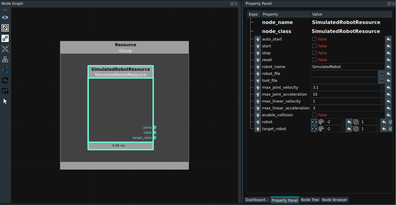
It is generally necessary to turn on the robot’s auto_start (automatic operation of robot resources) and open the robot’s visual properties. In addition, before running, you need to change the robot_file property to the robot rob file you need (you need to apply to the Tuyang technical support personnel in advance for the required robot digital model file). At the same time, if a tool such as a fixture and a suction cup is customized for the robot, it can be added to the ‘tool model’ property. Four attributes that control speed:

• max_joint_velocity：It is used to control the maximum joint speed of robot MoveJoints. Unit: radians per second.

• max_joint_acceleration：It is used to control the maximum joint acceleration of robot MoveJoints. Unit: radians per second squared.

• max_liner_velocity：It is used to control the maximum linear velocity of the robot in linear motion. Unit: meters per second.

• max_liner_acceleration：It is used to control the maximum linear acceleration of the robot in linear motion. Unit: meters per square second.

  Robot to run after the display of the picture as shown.

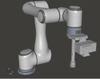
Robot control panel

Mouse Double click on the robot in 3D view, you can pop up the robot control panel:

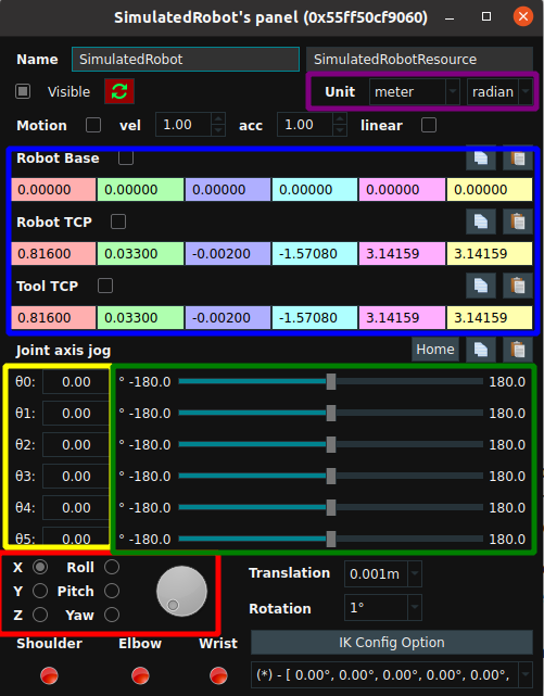
The robot joint Angle can be adjusted by entering the corresponding Angle in the joint value editing bar (yellow box above), or the robot joint rotation can be controlled by directly dragging the buoy on the right (green box above). You can also turn the knob to adjust the attitude x, y, z, rx, ry, rz, as shown in the red box above. All current pose values are displayed in the blue box above, and the display units can be adjusted (purple box above).

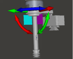
You can also actively control the robot to move to a certain position, and then check the posture at this time. First, click the Stop key in the upper left corner of the RVS software, and then check the ROBOT TCP in the blue box above. At this time, you can view the TCP pose at the end of the robot, as shown in the figure below. Drag these arrows on the diagram to move the whole robot. The robot attitude information during movement can be consulted in the control panel at any time.

The simulation movement of robot is controlled by node

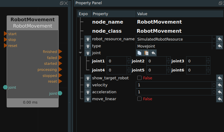
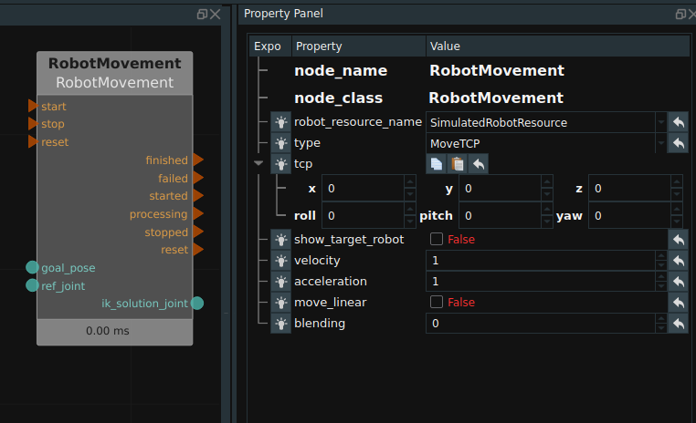
In the actual use of the project, the target pose is often known, and the robot needs to be moved to the past for simulation display. At this point you can use MoveTCP node in RobotMovement, as shown in the figure below. When used, the joint coordinates before the robot moves need to be connected to the left ref_joint, and the target pose (or pose list) to be moved needs to be connected to the left goal_pose. After the operation is completed, the joint coordinates after the robot moves are output to the right ik_solution_joint. The velocity and acceleration properties of the node can be adjusted to adjust the velocity and acceleration of the node’s current motion. Adjust the linear motion property to determine whether the motion is linear.

If you know the joint coordinates that the robot needs to move to a certain position, you can use the MoveJoint node in RobotMovement. When used, the joint coordinates that the robot needs to move need to be connected to the left joint.